1  Quality Check

Week 1 - Quality checks and data exploration

In this first workshop, we’ll introduce you to R, RStudio, and the basics of coding. You’ll be writing your first lines of R code and importing data today! Workshop materials are available in the github repository ECS200.

Before we start

This step can be skipped if you have R and Rstudio already downloaded and installed.

Murdoch computer

All Murdoch computers have R and Rstudio available. Login to your account and access Rstudio on your work computer.

Your own computer

If you are using your own personal computer in this unit, here are the steps for downloading and installing R and Rstudio.

1. Install R
   • Go to https://cran.r-project.org
   • Choose your operating system and follow the instructions to install.
2. Install RStudio
   • Go to https://posit.co/download/rstudio-desktop/
   • Download the free version of RStudio Desktop.
   • Install it on your computer.

Step 1: Open RStudio

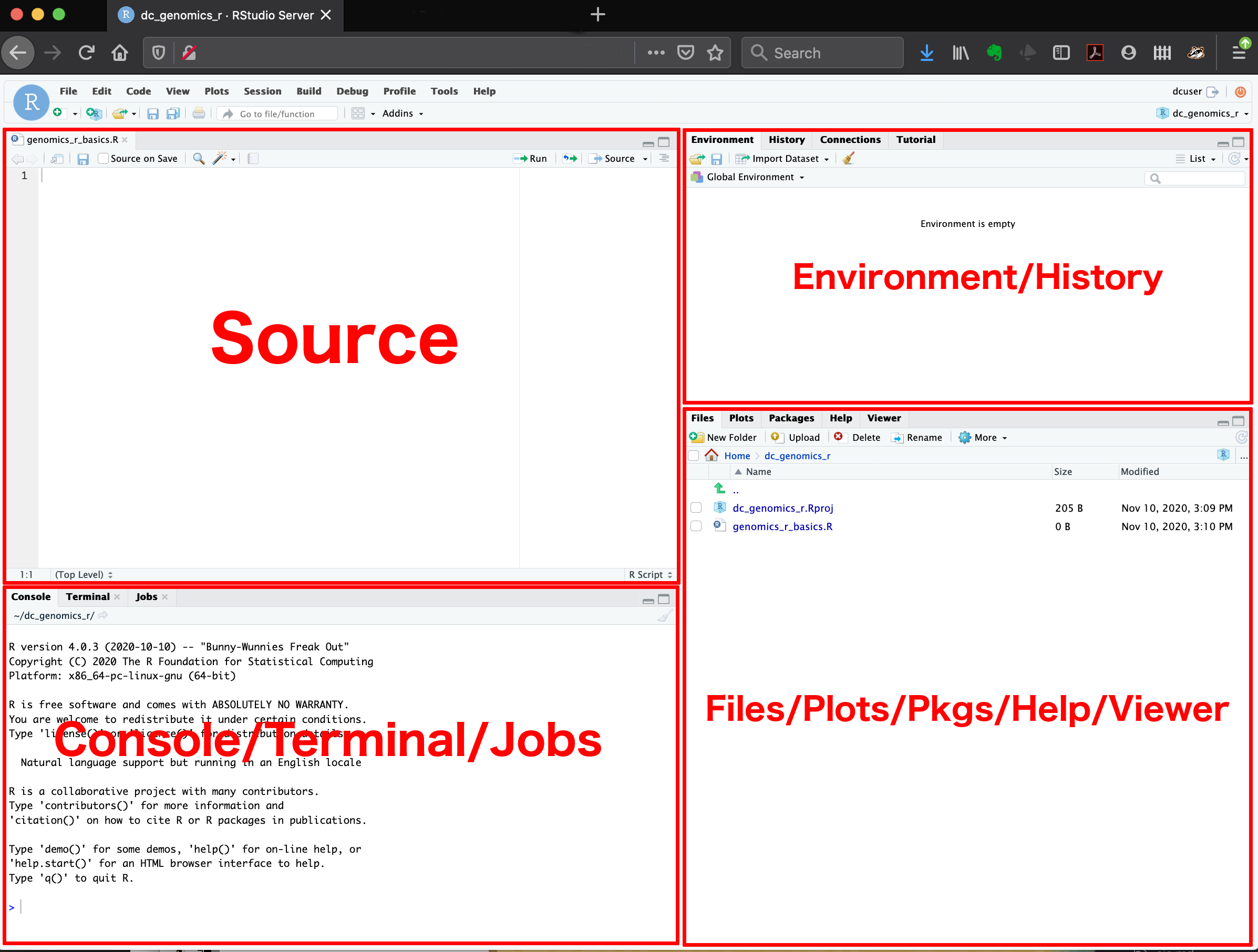
Once you have opened RStudio, you are introduced to the interface where you can see four panels:

• Console: Where commands run.
• Source: Where you write and save your code.
• Environment/History: See your datasets and objects (variables) and previous commands (“History” tab).
• Plots/Packages/Help/Files: View graphs and manage tools. You can also use the “Files” tab to navigate and set the working directory. The “Plots” tab will show the output of any plots generated. In “Packages” you will see what packages are actively loaded, or you can attach installed packages. “Help” will display help files for R functions and packages. “Viewer” will allow you to view local web content (e.g. HTML outputs).

Fig. 1. Layout with the four major windows (or panals) of the RStudio environment.

Step 2: First R Commands

Click File > New File > R Script to start.

Start by noting who is writing, the date, and the main goal. In our case, determining how many species from different taxa have been recorded in Perth Here’s an example, which you can copy, paste and edit into your new script and change the content:

# Week 1 workshop - Getting started
# Getting familiar with R and load a file
# Written by Nicholas Wu, 06/11/2024, Murdoch University

The # (hash/pound) is to tell R to not run this line of text. i.e., the comment will not be evaluated. Typically, the # is used to annotate or give explanation for what the code is doing.

Note: Comment often and in detail. Someone should be able to understand what you did and why. Including your future self.

Let’s try typing and running some code. Type the following code blow into the ‘source’ window (Fig. 1) and run each line so it shows up in the ‘console’ window:

# Create a variable: number of frogs counted at a pond
frogs <- 18

# Add 5 frogs observed the next day
frogs_total <- frogs + 5

# Print result
frogs_total

# You can now do additions in R with variables!

Here, you can created a new object frogs with the assignment operator “<-”. object_name <- value

Try this one too which creates a list of numbers assigned to the variable leaf_sizes, and then calculates the mean value of this list:

# Mean leaf size of 5 Eucalyptus trees (cm²)
leaf_sizes <- c(23.4, 21.8, 25.1, 19.7, 22.5)

# Calculate the average leaf size using the mean() function
mean(leaf_sizes)

# You can can how create objects (leaf_size) that contain variables (23.4, 21.8, 25.1, 19.7, 22.5) in R!

You can combine multiple elements into a vector¹ with c().

Exercise (1 min)

🧪 Challenge: How would you find the largest leaf size?

Use the max() function.

Show answer

max(leaf_sizes)

Step 3: Loading Packages

The next few lines of code usually load the packages you will be needing for your analysis. A package is a bundle of commands that can be loaded into R to provide extra functionality. For example, you might load a package for formatting data, or for making maps.

To install a package, type install.packages("package-name"). You only need to install packages once, so in this case you can type directly in the console box, rather than saving the line in your script and re-installing the package every time.

Once installed, you just need to load the packages using library(package-name). Here, we will load the most common packages we will be using in this unit.

The next lines of code should define your working directory. This is a folder on your computer where R will look for data, save your plots, etc. To make your workflow easier, it is good practice to save everything related to one project in the same place, as it will save you a lot of time typing up computer paths or hunting for files that got saved R-knows-where.

For instance, you could save your script and all the data for this tutorial in a folder called “Intro_to_R”. It is good practice to avoid spaces in file names as it can sometimes confuse R. For bigger projects, consider having a root folder with the name of the project (e.g. “My_PhD”) as your working directory, and other folders nested within to separate data, scripts, images, etc. (e.g. My_PhD/Chapter_1/data, My_PhD/Chapter_1/plots, My_PhD/Chapter_2/data, etc.)

To find out where your working directory is now, run the code getwd(). If you want to change it, you can use setwd(). Set your working directory to the folder you just downloaded from GitHub:

# Install packages using the install.packages() function.
install.packages("tidyverse")

# Load the tidyverse package
library(tidyverse)

# This is an example filepath. Change the quoted area to your own filepath
setwd("C:/User/CC-1-RBasics-master")

Note

There are quotation marks when installing a package, but not when loading it.

Note

For windows, the copied file directory will use  but R does not recnonigse this. Replace  with / instead.

Step 4: Loading Files

Imagine we’ve collected leaf-trait data to look at the growth of seedlings from untreated (control) and calcium-treated sites. The additional calcium is hypothesised to increase the growth of the seedlings. The file is called plant_calcium.csv from the GitHub page. The original data with background explanation of the study is linked here.

First, save the file from the GitHub page to your RStudio project folder (wherever you set your directory). The plant_calcium.csv is in the ‘data’ folder.

# Load a CSV file
#plant_calcium_data <- read_csv("https://raw.githubusercontent.com/nicholaswunz/ECS200-Workshop/refs/heads/main/data/plant_calcium.csv")

# Here is an example working directory from my folder, remember to replace with yours.
setwd("C:/Users/75002992/OneDrive - Murdoch University/Teaching/ECS200 - Research Methods in Ecology/ECS200-Workshop/data") 

# Load a CSV file and give it an object name called plant_calcium_data
plant_calcium_data <- read_csv("data/plant_calcium.csv")

# View the first few rows of plant_calcium_data
head(plant_calcium_data)

# Displays the last rows of plant_calcium_data
tail(plant_calcium_data) 

 # Tells you whether the variables are continuous, integers, categorical or characters (see Exploring data below)
str(plant_calcium_data)
glimpse(plant_calcium_data)

# num or <dbl> means number values
# chr or <chr> means character values

Note

Remember to save your script once in a while! If you haven’t saved it already, why not save it in the same directory as the rest of the tutorial file, and give it a meaningful name.

Step 5: Exploring the Data

str(object.name) is a great command that shows the structure of your data (atomic class). So often, analyses in R go wrong because R decides that a variable is a certain type of data that it is not. For instance, you might have four study groups that you simply called “1, 2, 3, 4”, and while you know that it should be a categorical grouping variable (i.e. a factor), R might decide that this column contains numeric (numbers) or integer (whole number or count) data. If your study groups were called “one, two, three, four”, R might decide it’s a character variable (words or strings of words), which will not get you far if you want to compare means among groups. Bottom line: always check your data structure!

Class	Description	Examples	Use
numeric	These are numbers that can take any value within a range (continuous).	3.14, -2.5, 100.5	Height, weight, temperature.
integers	Whole numbers without decimal points.	1, 10, 100, 0, -42	Counting items, indexing.
factors	Variables that take on a limited number of distinct values (categorical).	“low”, “medium”, “high” or “male”, “female”	Grouping data, statistical modeling.
character	Text data.	“apple”, “hello world”	Names, labels, descriptions.

You can see that when you run str(plant_calcium_data), each column has the name of the varliable and the class type next to them. For example, year is a num class (numeric), elevation is a chr class (character) etc.

You’ll notice the watershed variable shows as a character variable, but it should be a factor (categorical variable) consisting of a reference (untreated) category and a W1 (calcium-trated) category, so we’ll force it to be one. When you want to access just one column of a data frame, you append the variable name to the object name with a dollar $sign. This syntax lets you see, modify, and/or reassign this variable.

# Displays the first few rows of this column only (the reference group)
head(plant_calcium_data$watershed)

# Tells you what type of variable we're dealing with: it's character now but we want it to be a factor
class(plant_calcium_data$watershed)

# What are we doing here?!
plant_calcium_data$watershed <- as.factor(plant_calcium_data$watershed)

# check if watershed is now a factor
str(plant_calcium_data) # should say Factor
dplyr::glimpse(plant_calcium_data) # should say <fct>

In that last line of code, the as.factor() function turns whatever values you put inside into a factor (here, we specified we wanted to transform the character values in the watershed column from the edidiv object). However, if you were to run just the bit of code on the right side of the arrow, it would work that one time, but would not modify the data stored in the object. By assigning with the arrow the output of the function to the variable, the original plant_calcium_data$watershed in fact gets overwritten : the transformation is stored in the object. Try again to run class(plant_calcium_data$watershed) - what do you notice?

# More exploration

# Displays number of rows and columns
dim(plant_calcium_data)

# Gives you a summary of the data
summary(plant_calcium_data)

 # Gives you a summary of that particular variable (column) in your dataset
summary(plant_calcium_data$watershed) 

Note

Whenever you see an error like this:

library(ggrepel)
#> Error in library(ggrepel) : there is no package called ‘ggrepel’

You need to run install.packages("ggrepel") to install the package.

Part 2 - Quality Check

All statistical techniques have in common the problem of ‘rubbish in, rubbish out’

In this section, you will learn how to check the quality of the raw data you imported, and steps to correct errors in the raw data.

Background reading

How do we know the data is ready for analysis? Before we do any analysis, we need to check the raw data for the following:

• Check data structure and types: Use str() and summary() to ensure each column is the correct type (numeric, factor, character, etc.) and matches your expectations. e.g., Convert relevant character columns to factors for categorical analysis.
• Inspect for missing values: Use colSums(is.na() or visual tools (e.g., naniar::gg_miss_var() or visdat_viz_dat()) to identify missing data and decide how to handle it.
• Check for duplicates: Ensure there are no unintended duplicate rows or IDs.
• Validate categorical variables: Confirm that categories are consistent and correctly formatted (e.g., all lower case, no extra spaces).
• Scan for outliers or impossible values: Look for values outside expected ranges (e.g., negative stem lengths, impossible dates).
• Review column names: Ensure column names are meaningful, have no spaces or special characters, and are consistent.
• Preview the data: Use plotting functions to visually inspect the data for obvious issues.
• Check for extra rows or columns: Sometimes, files have summary rows, notes, or empty columns that should be removed.

These steps help ensure your data is reliable, interpretable, and suitable for statistical analysis. Importantly, it makes you a trustworthy researcher!

Before we start

Create a new R file. You don’t need to save the previous one. Click File > New File > R Script to start. Write the workshop name, the main goal and your name and date. Always do this when starting a new script.

# Week 1 workshop - Getting started
# Getting familiar with R and load a file
# Written by Nicholas Wu, 06/11/2024, Murdoch University

Exercise (5 min)

🧪 Get your workflow set up

Next, load your appropriate packages (the same tidyverse, and a one for visualising missing data called visdat at this stage), set your working directory via setwd(), and load the plant_calcium.csv via read_csv().

Lets call the imported data object plant_calcium_data this time.

Show answer

#install.packages("visdat")

library(tidyverse)
library(visdat)

# Load a CSV file
plant_calcium_data <- read_csv("YOUR-LOCAL-DIRECTORY/plant_calcium.csv")

Step 1: Data Quality Check

1.1. Initial check

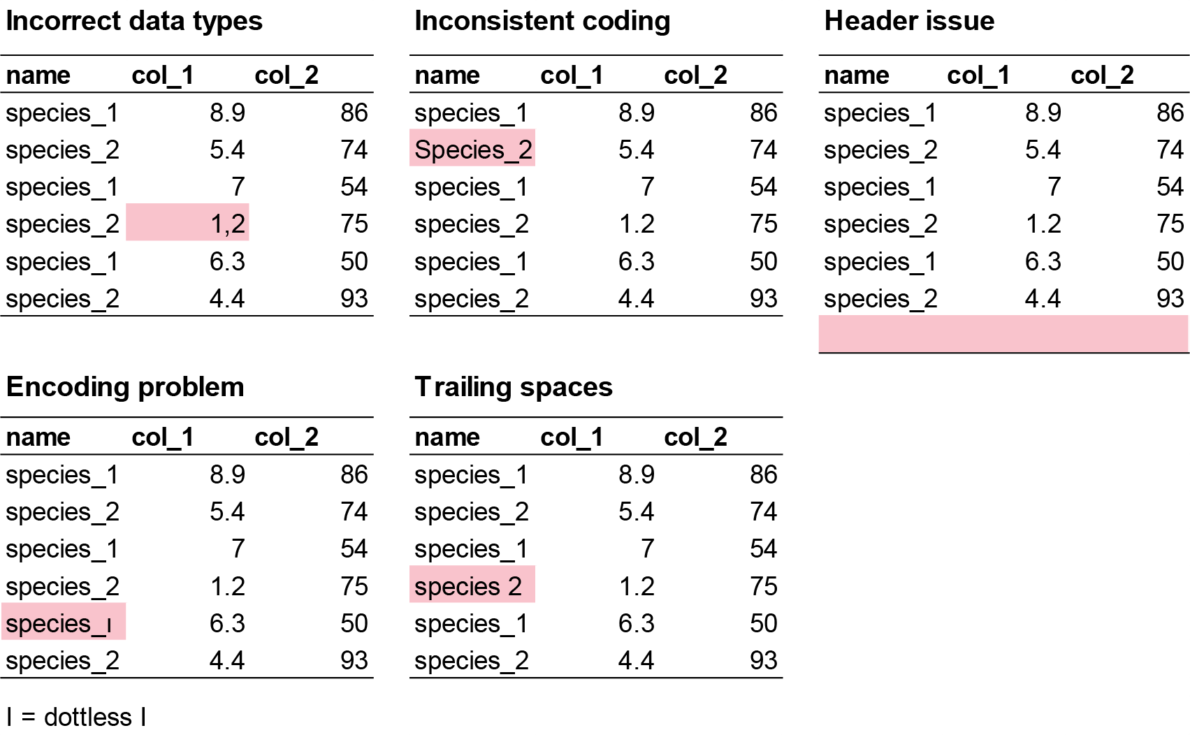
This helps you spot if variables are coded incorrectly (e.g., numbers as characters or vice versa), which could be due to the researcher error before inporting the data. Some example mistakes include:

• Incorrect data types: Numeric columns may be read as character (text) if there are unexpected symbols, missing values coded inconsistently, or formatting issues (e.g. a column meant to be numbers may contain text or empty strings, causing R to treat it as character instead of numeric).
• Inconsistent coding: Categorical variables may be inconsistently labeled (e.g., “Male”, “male”, “M”), leading to multiple categories that should be merged.
• Header issues: Sometimes, the header row is missing or duplicated, or extra non-data rows are included at the top or bottom of the file.
• Encoding problems: Special characters (e.g., accents, non-English letters) may not display correctly if the file encoding is not specified or mismatched.
• Trailing spaces: Spaces at the start or end of strings can create unexpected categories or prevent proper matching.

For small datasets (like in this workshop) it is easier to make fixes directly from Excel and import the new .csv file. As before, we will check the data here first with the str() function.

# Check the structure of your data
str(plant_calcium_data)
glimpse(plant_calcium_data)

# Get a summary of all variables
summary(plant_calcium_data)

If you would like to change the mistake in R directly, here is the code to do so using the recode() function. For example, let’s say you have three sites called A, B, C, but you noticed one site was mistakenly labelled as E. Here is how to change “E” to “B”.

fake_data <- data.frame(
  site = c("A","A","A","B","E","B","C","C","C"),
  species_1 = c(3, 7, 5, 2, 9, 4, 6, 1, 8)
)

fake_data %>%
  mutate(site = recode(site, "E" = "B")) # recode order by providing the variable you want to change "E", and the new variable name "B".

Let’s say you have a character that is suppoose to be a numeric value. e.g. “nine” instead of “9”, you will do the same thing as above but convert ‘chr’ to ‘num’ using as.numeric() function.

# Create fake data
fake_data <- data.frame(
  site = c("A","A","A","B","E","B","C","C","C"),
  species_1 = c(3, 7, 5, 2, "nine", 4, 6, 1, 8)
)


# Create a new object called fake_clean_data that replaces 'nine' with '9' and chnage species_1 to numeric
fake_clean_data <- fake_data %>%
  mutate(species_1 = recode(species_1, "nine" = "9"),
         species_1 = as.numeric(species_1))

# check if species_1 is numeric in the new fake_clean_data
glimpse(fake_clean_data)

Exercise (5 min)

🧪 Find the incorrect class in this dataset

I have created an example dataset called fake_data with three things wrong with it. Find the three issues in this dataset.

fake_data <- data.frame(
  site = c("A", "B", "C", "A", "B", "A", "B", "C", "a", "B", "A", "B", "A", "B", "C", "C", "B", "A", "A", "C", "B", "C", "C", "A", "A", "A", "A", "B", "C", "C", "C"),
  species_1 = c(7, 25, 30, 50, 38, 13, 5, 31, 34, 22, 41, 25, 22, 37, 39, 13, 45, 10, 40, 7, 28, 36, 19, 2, 12, 5, 16, 38, 27, 44, 44),
  species_2 = c(9.3, 8.6, 0.8 , 7.5, 9 , 9.1, 4.3, 8.6, 0.1, 7.8, 1.2, 6.2, 0.4, 0.4, 7.4, 1.9, 8.3, 7.8, 2.9, 9.3, 9.1, 2.3, 6.3, 8.5, 6.5, 6.6, "1,7", 1.8, 8.4, 4.7, 4.7),
  species_3 = c(190, 160, 70, 430, 310, 99, 530, 420, 371, 357, 198, 171, 463, 124, 254, 484, 435, 409, 122, 305, 410, 162, 473, 200, 401, 273, 421, 419, 293, 487, 487),
  species_4 = c(2, 0, 4, 8, 6.7, 3, 7.2, 4.3, 2, NA, 10, 10, 6, 4, 8, 1.7, 1, 0, NA, 4, 6, 8.2, 10, 6, 2, 5, 10, 7, NA, NA, NA)
)

What are the identified issues?

Show answer

1. site should be factor, not character
2. species_2 should be numeric, not character
3. species_4 has 5 NA’s

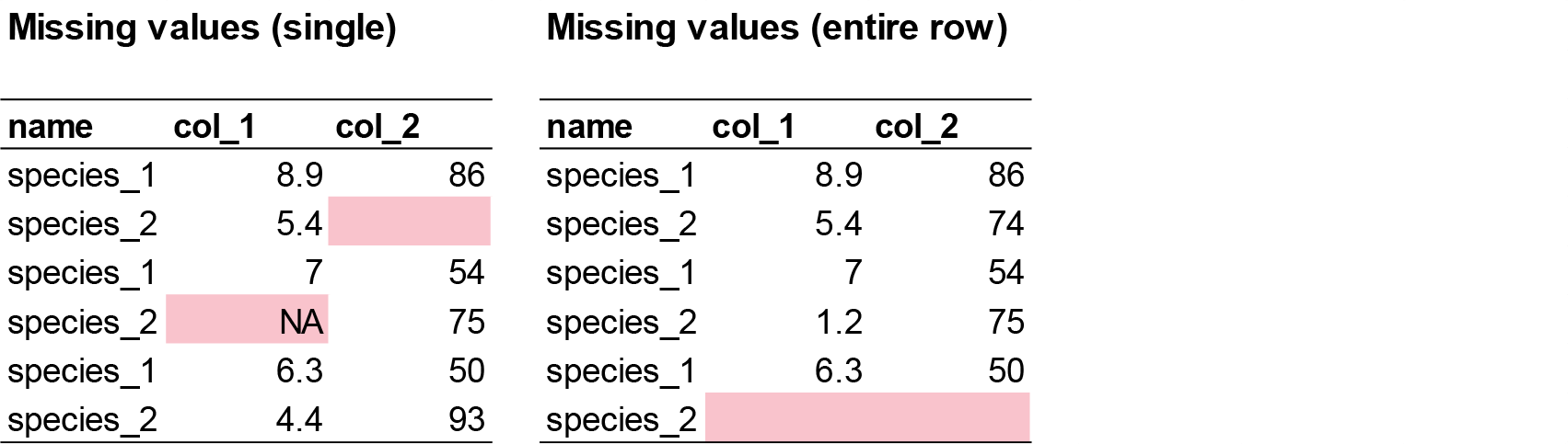
1.2. Identify missing values

Missing data may appear as blanks, “NA”, “.”, or other placeholders. If not handled properly, this can cause errors or misinterpretation during analysis.

# Check for missing values in each column
colSums(is.na(plant_calcium_data))

# Visualise missing data pattern
visdat::vis_dat(plant_calcium_data)

vis_dat() visualises the whole dataframe at once, and provides information about the class of the data input into R, as well as whether the data is missing or not.

The function vis_miss() provides a summary of whether the data is missing or not. It also provides the amount of missings in each columns.

# Visualise missing data pattern
visdat::vis_miss(plant_calcium_data)

Option: Removing columns with missing values

# Removes all rows with NA in the dataset
plant_data_clean <- plant_calcium_data %>% 
  drop_na()

# not recommended if NA is scattered across columns (e.g. leaf1area) because some important variables might be dropped out.

# If you only want to drop rows where NA is present in the elevation column only.
plant_data_clean <- plant_calcium_data %>% 
  drop_na(elevation)

# Run the vis_miss again on the clean data to check if the NA rows are removed. 
visdat::vis_miss(plant_data_clean)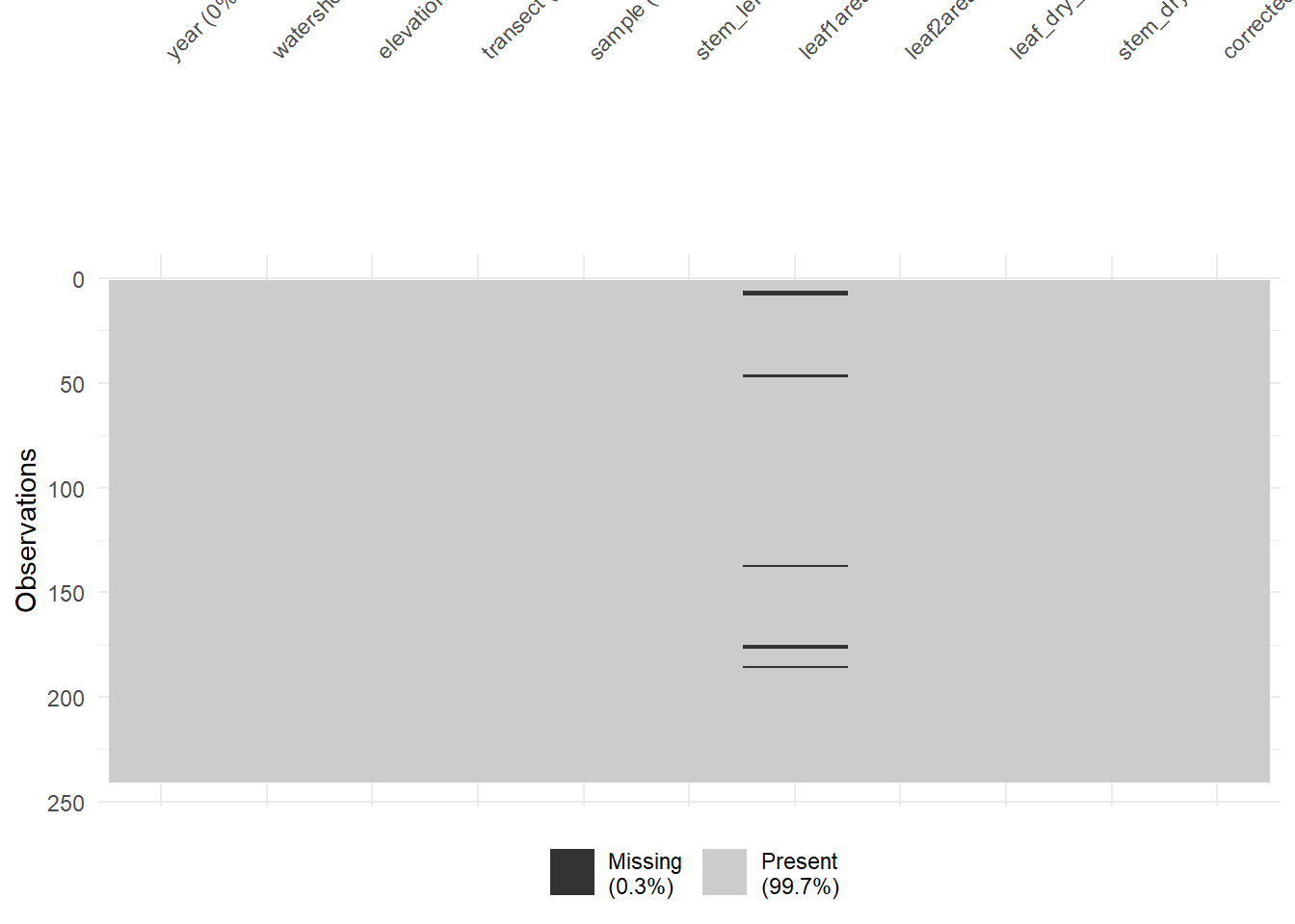

Exercise (5 min)

🧪 Identify and handle missing values in the fake_data dataset

• Which column contains missing variables?
• How many missing values are there?
• Remove rows with missing values and create a new object called fake_data_clean.
• Visualise the new fake_data_clean with visdat::vis_dat(fake_data_clean).

Show answer

# Check for missing values in each column
colSums(is.na(fake_data)) # species_4, # 5 missing values

# Visualise missing data pattern
visdat::vis_dat(fake_data) 

# Drop rows where NA is present in the species_4 column only.
fake_data_clean <- fake_data %>% 
  drop_na(species_4)

# Run the vis_miss again on the clean data to check if the NA rows are removed. 
visdat::vis_miss(fake_data_clean)

1.3. Check for duplicates

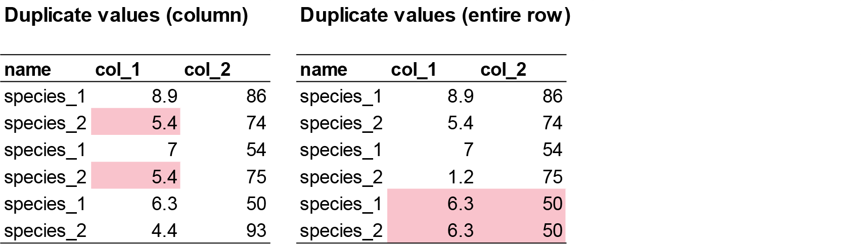
There are two common duplicate types that can happen in your dataset.

1. Row duplicates: where the values and names of two rows are identical 99% of the time, this is user error (e.g. copy pasted). These must be identified and removed.

sum(duplicated(plant_calcium_data))  # Returns the number of duplicate rows

# View the duplicate rows themselves
plant_data[duplicated(plant_calcium_data), ]

In the plant_calcium_data, there are no row duplicates.

2. Value duplicates: 90% of value duplicates in a column might be biologically realistic responses and is likely due to rounding of values during recording (e.g. values 2.5 and 2.5 might look duplicated due to user rounding. Actual values are 2.47 and 2.49). This is usually okay and can be kept in the dataset. User error occurs if there is a pattern in duplicates (e.g. 2,2,6,1,2,2,9,4,2,2,5,9). This can occur due to copy and pasting in the following row by accident.

You the researcher must decide whether these duplicate responses are real or due to user error.

sum(duplicated(plant_calcium_data$leaf_dry_mass))  # Returns the number of duplicate rows

plant_data[duplicated(plant_calcium_data$leaf_dry_mass) | duplicated(plant_calcium_data$leaf_dry_mass, fromLast = TRUE), ] # Returns all occurrences of duplicated numbers 

In the leaf_dry_mass column, there are 51 value duplicates.

Exercise (3 min)

🧪 Identify the duplicate row in the fake_data dataset

• Where is the duplicate row?
• Remove the duplicate row. Either manually in Excel (easy), or an R function (challenge).
• Are there other duplicate values and do you know if they are ecologically relevant duplicates (similar response) or user error?

Show answer

sum(duplicated(fake_data)) # 1 duplicate found

# View the duplicate rows themselves
fake_data[duplicated(fake_data), ] #1 duplicate row in row 31

sum(duplicated(fake_data$species_1))  # species_1 = 7
sum(duplicated(fake_data$species_2))  # species_2 = 6
sum(duplicated(fake_data$species_3))  # species_3 = 1
sum(duplicated(fake_data$species_4))  # species_4 = 15

Step 2: Visualising Data

2.1 Check for outliers

Outliers aren’t inherently “bad,” but they can cause problems depending on the context and goals of your analysis. They can:

1. Skew statistical results: A single extreme value can pull the mean far from the center, increase variability making data seem more spread than it really us, and can distrort the slope and intercept of linear models, leading to misleading predictions.
2. Create obscure patterns: Hide clusters or trends that would otherwise be visible.
3. Indicate user error: Data entry mistakes (e.g., typing 1000 instead of 100), measurement errors (e.g., faulty sensors), incorrect data merging (e.g., mixing units like metres and feet).

There are different ways we can check for outliers. See a more comprehensive page for more options. Here, we will create two common plots to check for outliers, and run some simple methods for detecting and removing outliers.

Boxplot

We can use the ggplot() function from the ggplot package to create a boxplot via geom_boxplot() showing the distribution of the lead2area data.

# Boxplot of leaf2area to detect potential outliers
ggplot(plant_data_clean, aes(y = leaf2area)) +
  geom_boxplot(fill = "lightgrey") +
  theme_bw()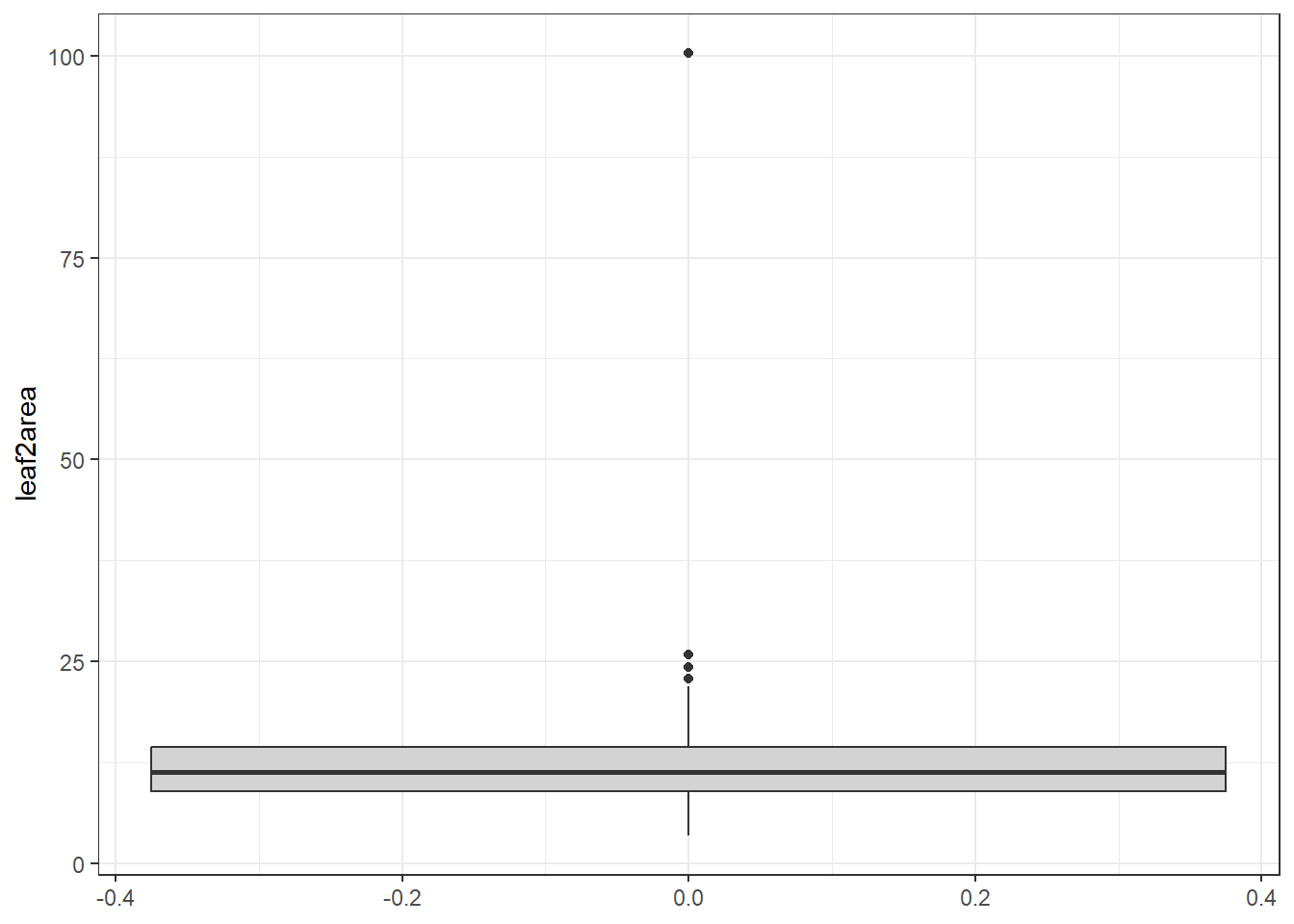

Histogram

Another way we can visualise outliers is with histograms via geom_histogram() or density plots via geom_density()

# Boxplot of height to detect potential outliers
ggplot(plant_data_clean, aes(x = leaf2area)) +
  geom_histogram() +
  theme_bw()

`stat_bin()` using `bins = 30`. Pick better value `binwidth`.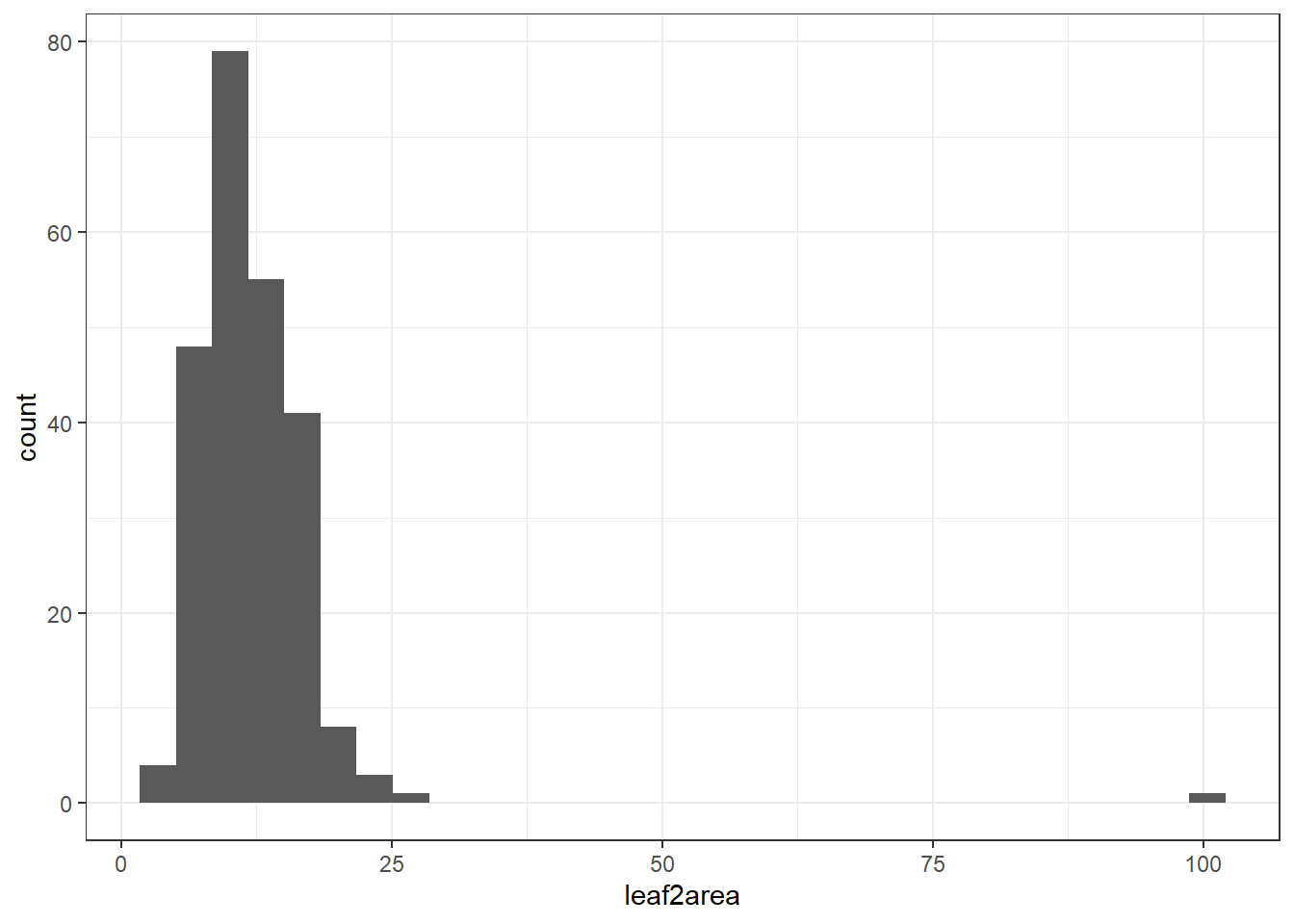

Here you can see one clear outlier with a value above 100. All other values are below 25. You can either manually remove the outlier on Excel, or with the following code below.

Option: Remove outliers using the interquartile range (IQR) rule.

# View potential outliers using IQR rule
Q1 <- quantile(plant_data_clean$leaf2area, 0.25, na.rm = TRUE)
Q3 <- quantile(plant_data_clean$leaf2area, 0.75, na.rm = TRUE)
IQR <- Q3 - Q1

# Filter rows with height outside 1.5 * IQR range
outliers <- filter(plant_data_clean, leaf2area < (Q1 - 1.5 * IQR) | leaf2area > (Q3 + 1.5 * IQR))
outliers

Make sure the numbers are biologically realistic based on intuition and comparing with the literature. If the values are unrealistic, it is a safe assumption to remove them.

2.2 Is the data normally distributed

This step is required to check if the data is suitable for certain types of analysis. Sometimes, transformation is required for certain data to meet the assumptions of certain statistical methods and improve the interpretability and performance of models. Many statistical techniques—like linear regression, ANOVA, and t-tests—assume that the data is normally distributed, has constant variance, and is linearly related (from your MAS183 - Statistical Data Analysis and MAS224 - Biostatistical Methods units). If the data is skewed, has outliers, or shows non-constant variance (heteroscedasticity), these assumptions are violated, which can lead to biased estimates, incorrect conclusions, or poor model fit.

By applying transformations such as logarithmic, square root, or Box-Cox, we can:

• Reduce skewness and make the distribution more symmetrical.
• Stabilise variance across levels of an independent variable.
• Improve linearity between variables.
• Minimise the influence of outliers.

Let’s check the distribution of leaf2area after removing that one outlier.

# remove values above 100
plant_data_clean <- plant_data_clean %>%
  filter(leaf2area < 100)

ggplot(plant_data_clean, aes(x = leaf2area)) +
  geom_histogram() +
  theme_bw()

`stat_bin()` using `bins = 30`. Pick better value `binwidth`.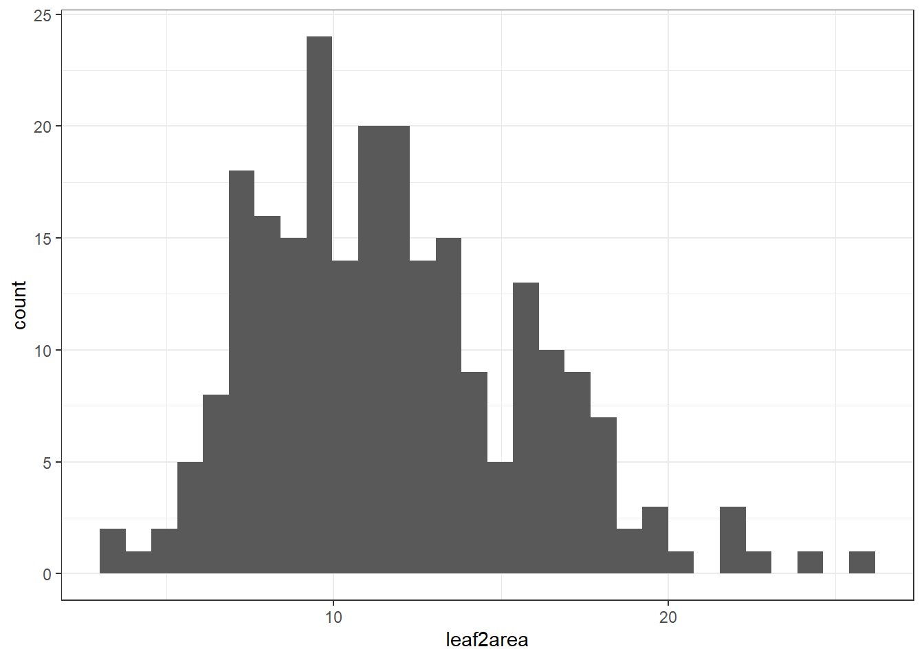

Looks normally distributed to me! We will learn data transformation in next weeks workshop.

Assessment

Part 1

Task to complete before the end of the workshop.

1. Create and manipulate variables:

• Create a variable called birds and assign it a value (e.g., number of birds seen).
• Create another variable called sites and a value between 2 and 10.
• Add a third observation and multiply the variables birds and sites to get the result in a new variable birds_total.

2. Work with vectors:

• Create a vector object called tree_heights with ten numeric values, or generate.
• Find the average tree height using the base R function.
• Find the minimum tree height using the base R function.

Note: You can use Google and ChatGPT to find the appropriate function. In the real world, you won’t be remembering every single function, but your skills in finding and using the right function will greatly help your career. In your future job, don’t just blindly cut and paste code to your R script. Understand why the code is presented and if it is relevant to your task. I’ve noticed AI models sometimes give extra code or takes unnecessary steps to get to the answer. Be efficient and comfortable with your code.

Optional - For the adventurous folks

For those comfortable with R and coding and would like an additional challenge. Here is a task for you before the next week.

• Create a vector tree_heights with 100 numeric values between 0-50 using the R random number generator.
• Find the quartile range of the from the tree_heightsvector.

Part 2

We will use a modified plant_calcium.csv dataset called plant_calcium_task.csv for the next workshop. Here, you need to conduct a quality check and data exploration of this new dataset and fix any potential issues. Download plant_calcium_task.csv from the GitHub page to your local folder (wherever you set your directory). The plant_calcium_task.csv is in the ‘data’ folder.

Set up your working directory and load the plant_calcium_task.csv to R and give it am object name. If you like, you can call it plant_task_data_raw.

To make it a bit easier for you, I have given you hints where the errors are so you dont have to look through every single column or every problem. But in your own dataset, you will need to thoroughly check your own data in the future.

Hints:

1. Identify missing values in one of the numeric columns. Remember to check if you really need to remove these missing value rows or not.
2. There is an inconsistent coding in one of the categorical variables. Correct the incorrect coding. You can do this on Excel, or from R (see adventurous folks section).
3. There are two numeric columns with outliers. One is biologically realistic, the other one is a data entry mistake. Decide which one is the data entry mistake and remove/correct that outlier.
4. Create a clean version of the data after removing the errors as plant_task_data_clean and visualise one of the numeric columns as a density plot.

When you have completed the assessment, save your plant_task_data_clean data as a csv file. The plant_task_data_clean should have the NA’s and outliers removed, and watershed transect changed to factor.

Here’s how to do it in R with write.csv(). The location of the saved file should be your working directory.

write.csv(plant_task_data_clean, file = "plant_task_data_clean.csv")

Optional - For the adventurous folks

Here we will start thinking about writing code efficiently. For example, you would have noticed by now that whatever raw data we load in R, any categorical columns are automatically listed as characters. So you can write a code that both loads the data and change the characters to factors in the same line of code (e.g. using the dplyr::mutate() function). Load the plant_calcium_task.csv and change categorical variables from character and factor.

Repeat the same assessment as above, but instead of correcting the errors by editing them on Excel, do all the corrections within the R environment. Visualise the clean version of the the data with a density plot but separate the density by the treatment groups (reference and W1 variables).

Extra Stuff

Why is my code not working!

Computers are only as smart as the humans that use them.

If your code is not working there is most likely a spelling mistake or a typographic error. These human errors are easy to miss but equally easy to fix!

If your code is not working take a moment to breathe. Then check for common, minor errors such as:

• Spelling mistakes
• Wrong dataset name
• Wrong variable (column) name
• Missing or wrong quotation mark
• Missing bracket
• Inconsistent cases (e.g. Uppercase)
• Missed a step
• Invalid syntax (e.g. spaces)
• Duplicates of the same function with multiple errors – keep your scripts tidy!
• These reading/typing mistakes are the majority of encountered errors. They are not a big deal and are easily corrected.

You can and should easily fix the above mistakes yourself! We want you to know how to work problems out independently.

Exercise

🧪 Why does this code not work?

my_variable <- 10
my_varıable
#> Error: object 'my_varıable' not found

Look carefully! This may seem like an exercise in pointlessness, but training your brain to notice even the tiniest difference will pay off when programming.

Additional resource

• Loading other file types (if not .csv).
• How to rename factor levels in R.
• CrashCourse Statistics video on Plots, Outliers, and Justin Timberlake, with examples of went to remove outliers.

---

1. A vector is simply a list of items that are of the same type.