# If you need to install new packages, here are code hidden in the comments.
#install.packages("sf")

# Load libraries
library(tidyverse)
library(galah) # ALAs R package
library(sf) # work with spatial data9 OPTIONAL - Spatial Data
Week 9 - Plotting species observation data
This is an optional tutorial if you plan to work with species occurrence data.
Note
THIS TUTORIAL WILL NOT BE IN THE EXAM. It is an optional extra learning tool.
This tutorial contains examples occurrence spatial data, and was heavily inspired by Amanda Buyan and Dax Kellie’s tutorial from the Atlas of Living Australia.
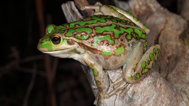
Maps are one of the most common and useful data visualisation tools in an ecologist’s tool belt. Making a quick and simple map of species observations is especially useful when first investigating where a species has occurred. Viewing locations of points can also help to understand the extent of your data (and spot possible errors or outliers). We will make a map of observations of the motorbike (Litoria moorei) in Western Australia since 2000 recorded by FrogID.
First, let’s load some packages.
Download the data
Search for taxa
When trying to download data about any species or clade, we can search using search_taxa(). It’s recommended to use search_taxa() to check whether a taxonomic search returns what you were expecting (even if you know the scientific name)! We can check taxonomic information about motorbike frog with search_taxa(), which returns extra details about the species when a match is found.
galah::search_taxa("Litoria peronii")# A tibble: 1 × 15
search_term scientific_name scientific_name_autho…¹ taxon_concept_id rank
<chr> <chr> <chr> <chr> <chr>
1 Litoria peronii Litoria peronii (Tschudi, 1838) https://biodive… spec…
# ℹ abbreviated name: ¹scientific_name_authorship
# ℹ 10 more variables: match_type <chr>, vernacular_name <chr>, issues <chr>,
# kingdom <chr>, phylum <chr>, class <chr>, order <chr>, family <chr>,
# genus <chr>, species <chr>Search for fields
Next, we can search for fields and field IDs for filtering our query. In this case, we are interested in filtering to a specific year, state/territory and data resource.
We can start by searching for any fields containing the word “year” using search_all().
galah::search_all(fields, "year")# A tibble: 8 × 3
id description type
<chr> <chr> <chr>
1 year Year fields
2 raw_year Year (unprocessed) fields
3 endDayOfYear End Day Of Year fields
4 startDayOfYear Start Day Of Year fields
5 occurrenceYear Date (by year) fields
6 raw_endDayOfYear <NA> fields
7 raw_startDayOfYear <NA> fields
8 namePublishedInYear Name Published In Year fieldsWe can do the same kind of search to find fields with information of australian states/territories and data resource names.
galah::search_all(fields, "states")# A tibble: 6 × 3
id description type
<chr> <chr> <chr>
1 cl2013 ASGS Australian States and Territories fields
2 cl22 Australian States and Territories fields
3 cl927 States including coastal waters fields
4 cl10925 PSMA States (2016) fields
5 cl11174 States and Territories 2021 fields
6 cl110925 PSMA States - Abbreviated (2016) fieldsgalah::search_all(fields, "resource")# A tibble: 5 × 3
id description type
<chr> <chr> <chr>
1 cl11160 Natural Resource Management (NRM) Regions 2023 fields
2 dataResourceUid Dataset fields
3 dataResourceName Dataset fields
4 relatedResourceID Related Resource ID fields
5 relationshipOfResource Relationship Of Resource fieldsIf you are ever uncertain which field ID to choose, you can use show_values() to see what possible values are within a field. For example, let’s see what values are in field ID cl22.
galah::search_all(fields, "cl22") %>%
  show_values()
• Showing values for 'cl22'.# A tibble: 11 × 1
cl22
<chr>
1 New South Wales
2 Victoria
3 Queensland
4 South Australia
5 Western Australia
6 Northern Territory
7 Tasmania
8 Australian Capital Territory
9 Macquarie Island
10 Coral Sea Islands
11 Ashmore and Cartier Islands Download observations
Now we are ready to build our query to download observations of motorbike frog in Western Australia since 2000 recorded by FrogID.
First, let’s find the number of records that match our query. This is good practice before downloading occurrence records because you can check exactly how many records you are intending to download (and avoid an accidental massive download)!
We’ll use atlas_counts() to download record counts, specifying the taxon using galah_identify(), and narrowing the year range, state/territory and data resource using galah_filter().
galah::galah_call() %>%                          # Begin a query
  galah::galah_identify("Litoria moorei")  %>%   # motorbike frog
  galah::galah_filter(year >= 2000,              # since 2000
               cl22 == "Western Australia",      # in Western Australia
               dataResourceName == "FrogID") %>% # by FrogID
  galah::atlas_counts()
# A tibble: 1 × 1
count
<int>
1 7751Now we can use atlas_occurrences() to download occurrence records, which returns each observation’s location coordinates and event date.
You will need to first provide a registered email with the ALA using galah_config() before retrieving records.
galah_config(email = "your-email-here")frogs <- galah::galah_call() %>% # Begin a query
galah::galah_identify("Litoria moorei") %>% # motorbike frog
galah::galah_filter(year >= 2000, # since 2000
cl22 == "Western Australia", # in Western Australia
dataResourceName == "FrogID") %>%
galah::atlas_occurrences()Request for 7751 occurrences placed in queue.Current queue length: 1--frogs# A tibble: 7,751 × 9
recordID scientificName taxonConceptID decimalLatitude decimalLongitude
<chr> <chr> <chr> <dbl> <dbl>
1 00006222-be99… Litoria moorei https://biodi… -31.9 116.
2 0010a4bf-3221… Litoria moorei https://biodi… -31.9 116.
3 00120d3d-fcf8… Litoria moorei https://biodi… -31.8 116.
4 001528f5-e4ed… Litoria moorei https://biodi… -33.4 116.
5 0025e663-0b68… Litoria moorei https://biodi… -32.1 116.
6 002a0df6-3b6e… Litoria moorei https://biodi… -31.9 116.
7 002b6785-6dcf… Litoria moorei https://biodi… -31.9 116.
8 002d8daa-be17… Litoria moorei https://biodi… -31.9 116.
9 00423fd5-85c2… Litoria moorei https://biodi… -31.9 116.
10 005e6056-a7a5… Litoria moorei https://biodi… -31.9 116.
# ℹ 7,741 more rows
# ℹ 4 more variables: eventDate <dttm>, basisOfRecord <chr>,
# occurrenceStatus <chr>, dataResourceName <chr>Make a map
It’s time to make our map!
Let’s load our States and Territories shapefile from the ozmaps R package. Then, we will filter the shapefile to Western Australia and quickly plot it to check it plots correctly (specifying that the border is grey, and the inside is white).
library(ozmaps)Warning: package 'ozmaps' was built under R version 4.5.3au_map <- ozmaps::ozmap_data("abs_ste")
WA_map <- au_map[au_map$NAME == "Western Australia",]
ggplot() +
geom_sf(data = WA_map,
colour = "grey60",
fill = "#F5F5F5") +
theme_bw()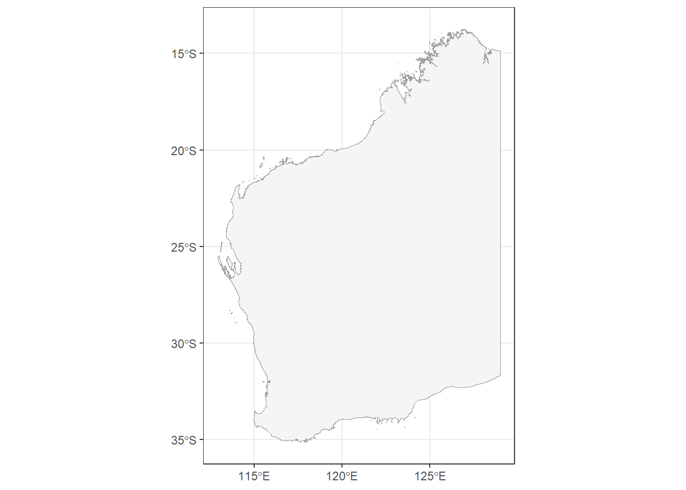
Our shapefile has plotted nicely, but there are many different ways to display our shape of WA, which exists on a spherical globe (the Earth), onto a flat surface (our map). Our shapefile already has a projection, determined by its Coordinate Reference System (CRS) of GDA94.
sf::st_geometry(WA_map)Geometry set for 1 feature
Geometry type: MULTIPOLYGON
Dimension: XY
Bounding box: xmin: 112.9211 ymin: -35.18823 xmax: 129.002 ymax: -13.68879
Geodetic CRS: GDA94MULTIPOLYGON (((114.4178 -22.31538, 114.414 -22...To make it clearer how the CRS changes the projection of a map, here are 3 maps of NSW projected with 3 different CRS:
GDA94 (the current projection of our NSW shapefile)
EPSG:7850 (a state/territory-specific projection for WA)
EPSG:2955 (intended for Canadian territories)
library(cowplot)

p1 <- WA_map %>%
  ggplot() +
  geom_sf(colour = "grey60",
          fill = "#F5F5F5") +
  labs(title = "GDA94") +
  theme_bw()

p2 <- WA_map %>%
  st_transform(crs = st_crs(7850)) |>
  ggplot() +
  geom_sf(colour = "grey60",
          fill = "#F5F5F5") +
  labs(title = "EPSG:7850") +
  theme_bw()

p3 <- WA_map %>%
  st_transform(crs = st_crs(2955)) |>
  ggplot() +
  geom_sf(colour = "grey60",
          fill = "#F5F5F5") +
  labs(title = "EPSG:2955") +
  theme_bw()

cowplot::plot_grid(p1, p2, p3, align = "h", nrow = 1)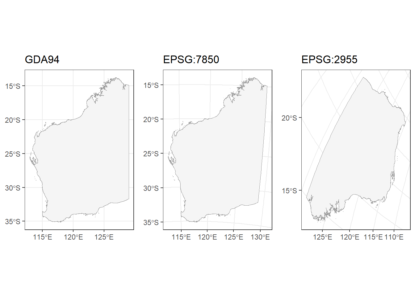
Now, we will add species observations to our map. First, we will plot our shapefile. Then, we will overlay a scatter plot using decimalLongitude as your x axis and decimalLatitude as your y axis. We’ll set the colour and adjust the alpha to make our points partially transparent.
ggplot() +
  geom_sf(data = WA_map,
          colour = "grey60",
          fill = "#F5F5F5") +
  geom_point(data = frogs,
             aes(x = decimalLongitude,
                 y = decimalLatitude),
             colour = "#6fab3f",
             alpha = 0.5,
             size = 1.1) +
  theme_bw()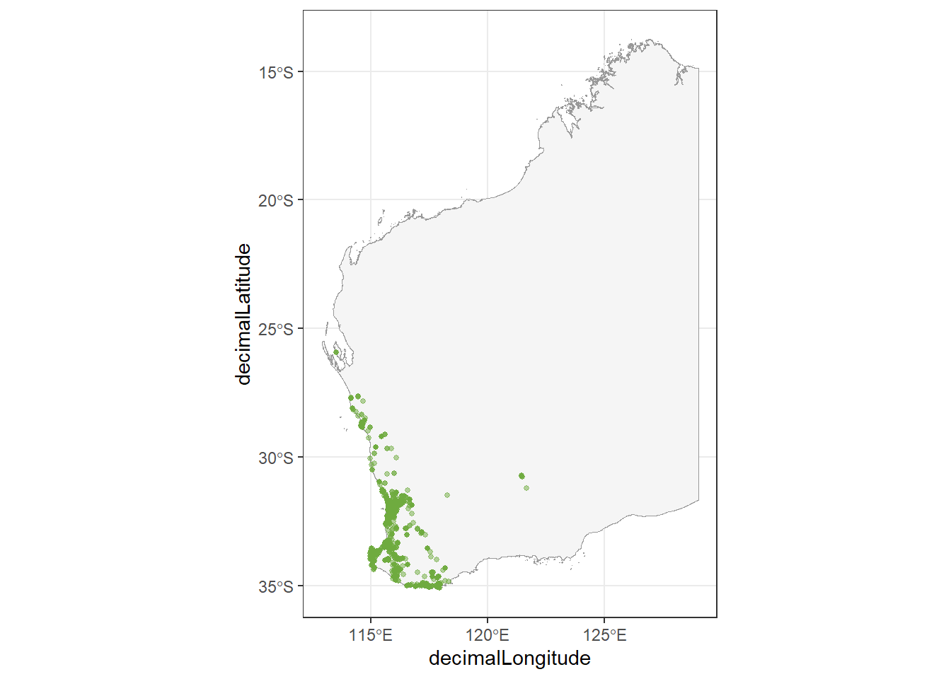
Density
We can use the ggpointdensity package to visualise locations with many overlapping occurrences. With over 40,000 points plotted on our map, geom_pointdensity() allows us to see areas with higher densities of observations.
library(ggpointdensity)Warning: package 'ggpointdensity' was built under R version 4.5.3ggplot() +
geom_sf(data = WA_map,
colour = "grey60",
fill = "#F5F5F5") +
ggpointdensity::geom_pointdensity(data = frogs,
aes(x = decimalLongitude,
y = decimalLatitude),
alpha = 0.5,
size = 1.1) +
scale_colour_viridis_c(option = "viridis", # palette
direction = -1) + # reverse light-to-dark
guides(
colour = guide_colourbar(
title = "Number of\noverlapping\nobservations")
) +
theme_void()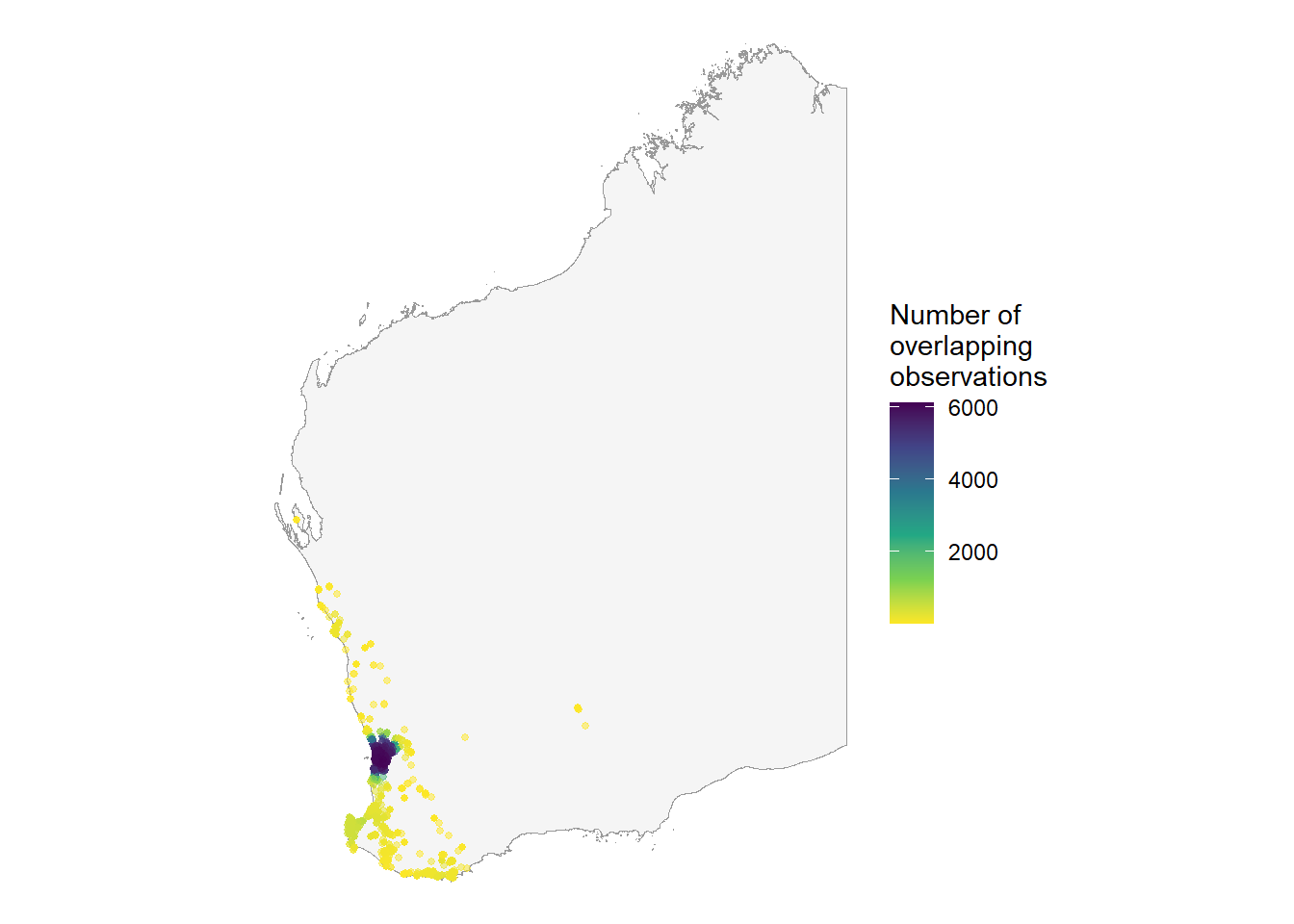
You can see most of the observations occur around the Perth metropolitan area.
Interactive map
You can also use the leaflet package to produce interactive maps:
#install.packages("leaflet")

library(leaflet)
Warning: package 'leaflet' was built under R version 4.5.3# convert to sf object and give crs 4326
frogs_sf <- sf::st_as_sf(frogs, coords = c("decimalLongitude", "decimalLatitude"), crs = 4326)
leaflet::leaflet() %>%
leaflet::addTiles() %>%
leaflet::addCircles(data = frogs_sf,
label = ~eventDate,
color = "#6fab3f")You can learn more about the leaflet package here. There is also a cheat sheet available here.
Learn more
Seasonality
Now we can make a bar chart or time series plot to see observations over the year.
# from the time-series tutorial
month_frogs <- galah::galah_call() %>%                         # Begin a query
  galah::galah_identify("Litoria moorei")  %>%  # motorbike frog
  galah::galah_filter(year >= 2000,             # since 2000
               cl22 == "Western Australia",     # in Western Australia
               dataResourceName == "FrogID") %>%
  galah::galah_group_by(month) %>%
  galah::atlas_counts() %>%
  mutate(month = lubridate::month(as.numeric(month), label = TRUE) # format month
         )

ggplot(data = month_frogs, aes(x = month, y = count)) +
  geom_bar(stat = "identity", fill = "#6fab3f") +
  labs(x = "Month",
       y = "No. of observations") +
  scale_x_discrete(expand = c(0,0)) +
  scale_y_continuous(limits = c(0, 1000),
                     expand = c(0,0)) +
  theme_bw()
Warning: Removed 4 rows containing missing values or values outside the scale range
(`geom_bar()`).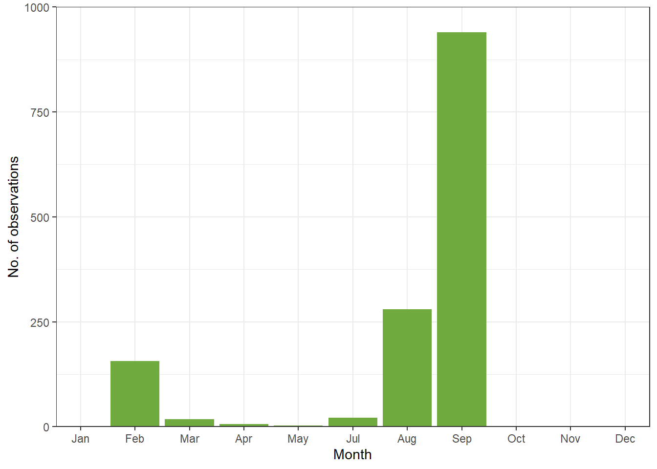
Important
Because the ALA database is based on both citizen and scientist submissions, recordings are not standardised and may be biased based on when people are aviabale to record such data, even for common species. For rare species, this is even more true. This type of time series plot for inferring seasonal activity or abundance over time is only reliable if you are standardising your survey across time. i.e no detection means you tried to look but they are not there vs not detected because you didnt survey in that time.
Cartographic data
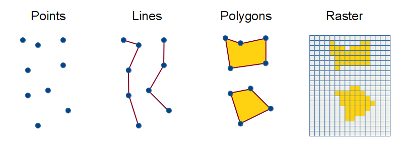
There are four main types of spatial cartographic data that R can handle. Cartographic data is represented by either vector or raster data.
Vector data is made up of points (x, y locations), lines (at least two connected points), and polygons (3 or more points that are connected and closed). These are used to represented discrete entities like survey plots/occurance (points), roads/rivers (lines), or boundary/country/lakes (polygons). How to best represent something depends on the scale at which the map will be shown.
Raster data is used to represent continuous information like rainfall or elevation per cell block (can be pixal size or actual units). These are phenomena that occur everywhere but to varying degrees. Each cell of the raster represents a numeric unit of data like feet above sea level.
This tutorial showed you how to load and plot point (ocuurance data) and polygon data (Western Australia map)
Analysis
You are now ready to analyse spatial data. However, spatial analysis is beyond this second-year unit, but here are some possibilities you can you do with spatial data:
Spatially-explicit regression models: This is your standard multilevel model but includes spatial distance between sites/populations as a covariance matrix in the model to account for similar responses in closely related sites. An example tutorial using a Baysian framework can be found here.
Species distribution modeling (environmental niche modelling): Uses algorithms to predict a species’ potential geographic distribution by relating known occurrence locations to environmental predictors (e.g., climate, soil, habitat). These models are crucial for conservation planning, climate change impact assessments, and invasive species management.
Movement ecology: Temporal and spatial data from tracking animals can help influence where animals move, how fast they move, if there daily/seasonal patterns in their movement, what kind kind of habitats do they move in, and what bahavioural states can be inferred from the data.
Additional resource
Cleaning Biodiversity data in R: A practical guide for cleaning geo-referenced biodiversity data using R. It focuses specifically on the processes and challenges you’ll face with biodiversity data.
Coding Club Working with Rasters and Remote-Sensing Data: An R tutorial to explore spatial analysis using satellite data to answer ecological questions such as what are the characteristics of species’ habitats.
Species distribution modelling using
tidysdm&tidymodels: An introduction to species distribution modelling with fundamental steps to build, assess and use models to predict species distributions.