data <- data.frame(ID = c(1, 2),
                   Jan = c(10, 20),
                   Feb = c(15, 25))

tidyr::pivot_longer(data, cols = Jan:Feb, names_to = 'Month', values_to = 'Value')3 Diversity Indices
Week 3 - Measurements of biodiversity
In this workshop, you will learn different types of ways to quantify diversity and abundance in your dataset. This section is particularly important for groups who are doing field studies, but this quantitative skill is also useful if you have a job in field ecology. Workshop materials are available in the github repository ECS200.
Background reading
Biodiversity can be measured using different scales and metrics, most commonly by looking at species richness (the number of different species) and species evenness (the relative proportion of individuals in each species). Other measurements include alpha, beta, and gamma diversity, which describe diversity within a single site, between sites, and across a larger region, respectively. Here, we will focus on the most common ways of quantifying diversity and abundance.
Abundance metrics
Absolute abundance (\(N_i\)): The total number of individuals of a species recorded. A simple and intuitive calculation, but sensitive to sampling effort, i.e, cannot compare across surveys without standardisation. Only use when sampling effort is standardised (e.g., same transect length, trap nights).
Relative abundance (\(p_i\)): Comparable across communities and is foundational for many diversity indices. Only use when communities have differing total abundance, or you need proportional representation, or over time.
Density (\(d_i\); individuals per area or effort): Allows spatial comparison, but requires accurate area/effort estimates. Appropriate for quadrat/plot/transect sampling.
Species richness metrics
Species richness (\(S\)): The total number of unique species. A sample and intuitive calculation, but highly sensitive to sample size and rare species. Only use when comparing equally-sampled plots or as a component in more complex metrics.
Rarefied richness: Standardised species richness for a fixed number of individuals or samples. Allows fair comparison across unequal sampling effort, but assumes random sampling, i.e low resolution when sample sizes differ greatly. Only use in surveys with unequal effort.
Diversity indices
Shannon diversity index (\(H'\)): Incorporates both species richness and evenness (the relative abundance of each species). Widely used, but difficult to interpret ecologically. Moderately sensitive to rare species, but good for comparing diversity across sites or time when both abundance and richness matter.
Simpson’s diversity index (\(D\)): Emphasises the dominance of species and is less sensitive to rare species. However, underweights rare species and may mask losses in low-abundance taxa. Use in management-focused studies (dominance effects), and stable community comparisons.
Other types of diversity metrics such as Rényi and Tsallis diversities, taxonomic diversity and taxonomic distinctness, alpha and beta diveristy can also be done with the vegan R package.
New functions
Here are some new functions from the tidyverse you will be using in this workshop.
pivot_longer()converts data from wide format to long format.starts_with()*used insideselect()to choose columns whose names begin with a specific string.across()* applies a function to multiple columns in asummarise()ormutate()call. e.g.everything()= select all columns andsum= function to apply..x* is a pronoun used inside anonymous functions in tidyverse pipelines—especially inacross()andmap(). It represents the current column being processed.
’*’ See ‘Relative abundance’ section for example use.
pivot_longer() converts wide data into long format. The function turns column names into values under a new variable.
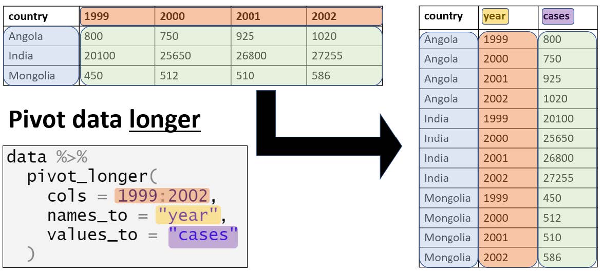
Example syntax in R:
pivot_wider() converts long data into wide format. The function spreads values across multiple columns using a key column. Useful when summarising tidy data.
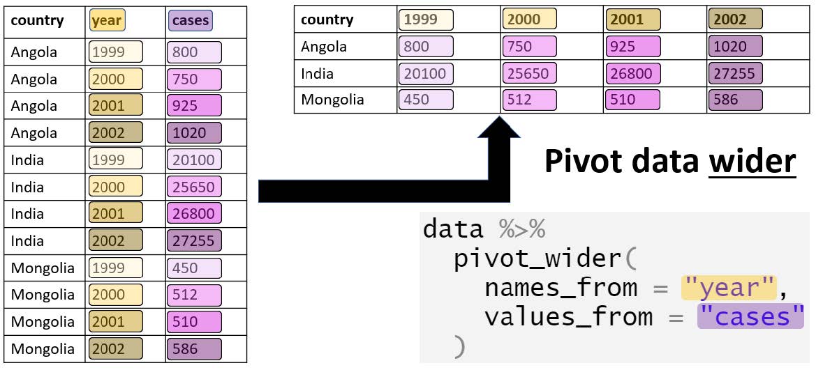
Example syntax in R:
data <- data.frame(
  ID = c(1, 1, 2, 2),
  Month = c('Jan', 'Feb', 'Jan', 'Feb'),
  Value = c(10, 15, 20, 25))

tidyr::pivot_wider(data, names_from = Month, values_from = Value)
cbind() combines dataframes by columns, binding them side-by-side. This function is used when data has the same number of rows and you want to add variables from a different dataset.
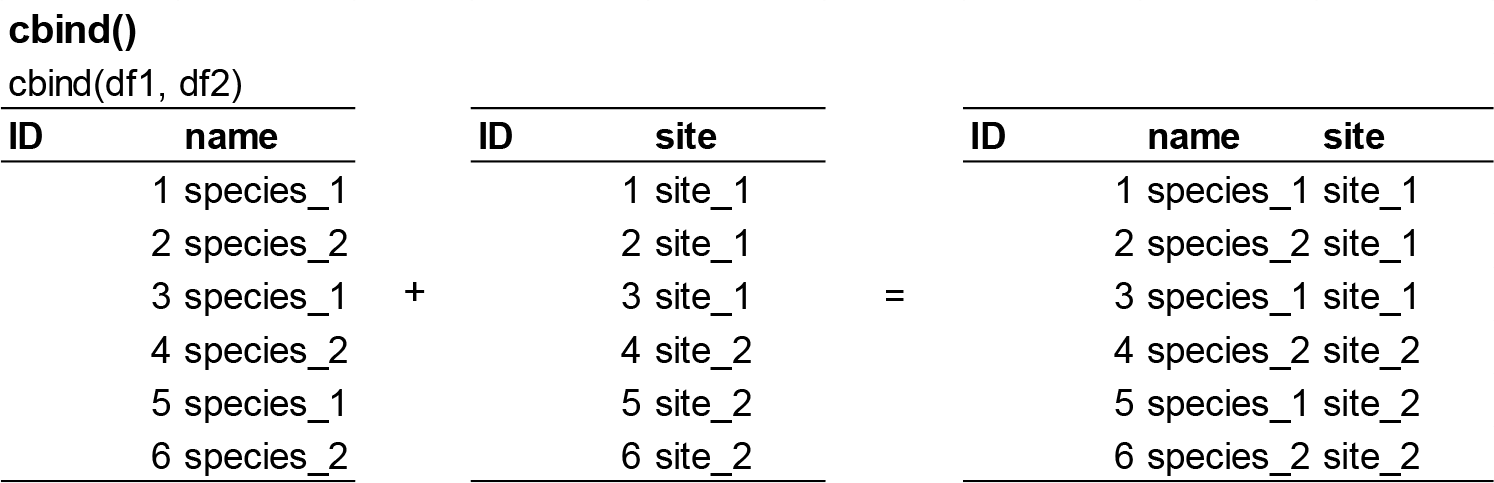
Example syntax in R:
# create two dataframes
df1 <- data.frame(ID = 1:3)
df2 <- data.frame(Name = c('A', 'B', 'C'))
# apply cbind() function
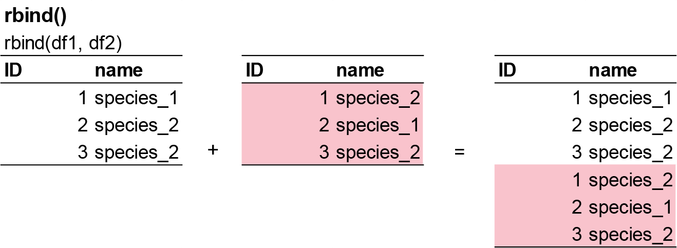
cbind(df1, df2)rbind() combines dataframes by rows, stacking them vertically. This function is used when data has the same columns and you want to add observations.
Example syntax in R:
# create two dataframes
df1 <- data.frame(ID = 1:2, Name = c('A', 'B'))
df2 <- data.frame(ID = 3, Name = 'C')

# apply rbind() function
rbind(df1, df2)
Zeros and NA’s in R
As mentioned previously, ecological data can be messy, but R does not care. rubbish in, rubbish out. When designing surveys for species observations, it is essential to distinguish carefully between ‘0’ and ‘NA’ in your data sheet, because they represent fundamentally different ecological and statistical realities.
A ‘0’ should be recorded only when a site was actually sampled with adequate effort and the species was truly not detected. In other words, sampling occurred, detection was possible, and the observed count was zero. As discussed by Blasco-Moreno et al. (2019) zeros can arise from different processes (e.g. true absence versus ecological or sampling processes generating excess zeros), and they carry biological meaning that will directly influence model choice and interpretation. A zero is data.
An ‘NA’, by contrast, should be used when the site was not sampled, sampling failed, effort was insufficient, or the observation is otherwise missing. An NA means “we do not know.”, or not collected not sampled.
The distinction matters greatly in R:
If you accidentally code a missing observation as ‘0’, you are asserting a confirmed absence. This can bias estimates of occupancy or abundance downward, inflate the number of zeros, distort mean–variance relationships, and potentially lead you to fit inappropriate models (e.g. zero-inflated models when the problem is actually missing data). For example, it makes no sense to replace it by zero if the entity was not recorded (e.g., if I didn’t measure pH in some samples because the pH-meter got broken, I should not replace these values by 0, since it does not mean that the pH of that sample is so low).
If you accidentally code a true zero as NA, R will drop that observation from many analyses (e.g. na.omit), reducing sample size and potentially biasing results if missingness is not random.
Different sources of zeros that could emerge in count data as seen in the figure below from Blasco-Moreno et al. (2019). The example shows the presence (>0) or absence (0) of herbivores on a plant species. Zeros due to the lack of experience of the observer (a–b) or resulting from a poor experimental design (c–h) are called False Zeros and should be minimized when performing the experiment. Structural Zeros, that is, zeros related to the ecological system under study (i–k), and Random Zeros emerging from the sampling variability (l) are known as True Zeros.
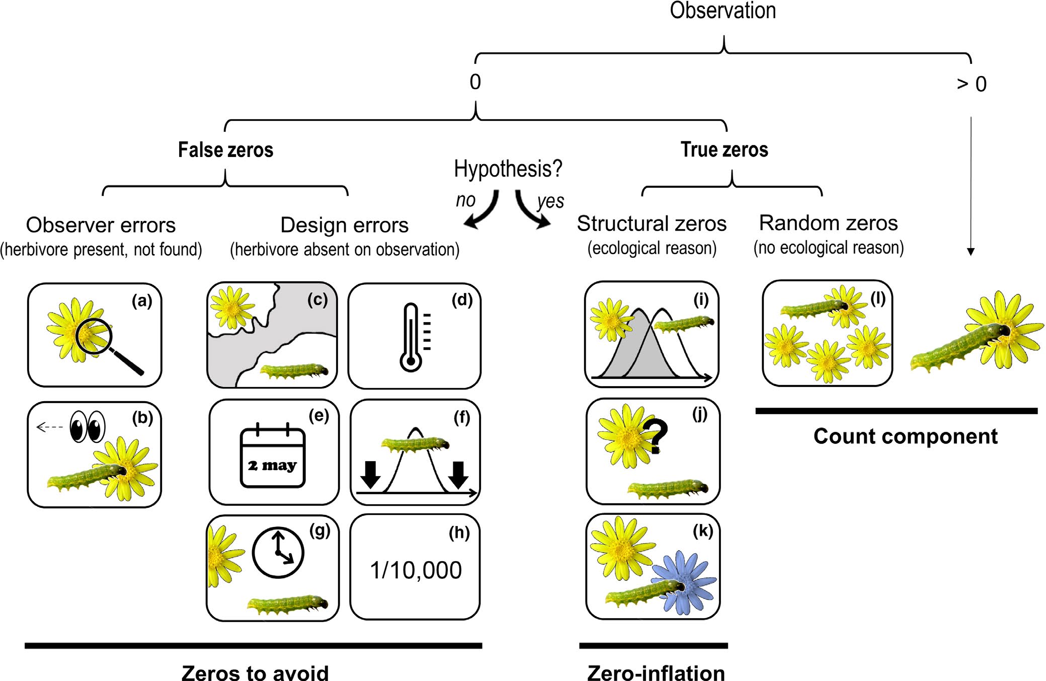
The following text explains different scenarios that would result in a zero value, and, in brackets, how errors due to false zeros can be minimized:
(a) the insects or the damage exerted are so small that the observer cannot detect them [sample when the insects are expected to be well developed];
(b) the observer does not see the herbivore (e.g. it is mistaken for a seed) or the damage is associated to other causes not related to herbivory (e.g. mechanical damage during sampling, pathogens, etc.) [the observer should be trained properly];
(c) the distributional areas of herbivores and plants are not coincident [know the species distribution before sampling];
(d) a herbivore is not present in a certain location within its distributional area, for example due to the microclimatic conditions [sample in habitats with adequate environmental conditions for a herbivore, or perform replicate surveys in different areas];
(e) a single survey is conducted, and is not coincident with the herbivore phenology [know the herbivore life cycle or perform long‐term surveys];
(f) a long‐term survey is conducted, but the low sampling frequency does not enable capture of the presence of the herbivore [sample on a more frequent basis];
(g) herbivores are not found because they are absent at the time of sampling [record plant damage instead of the presence of insects];
(h) herbivores are so infrequent that the design cannot capture their presence [perform extensive sampling with a high number of replicates];
(i) phenology of plants and herbivores are not completely coincident at a temporal level;
(j) herbivores do not recognize a plant as a potential host;
(k) herbivores recognize a plant as a host but prefer to feed on another species and
(l) the herbivore population is not large enough to saturate the available plant resources.
Calculations of abundance
We will start with this fake ecological survey data. Also, to calculate Shannon and Simpson’s diversity, we will need the the vegan package.
#install.packages('vegan')

# Load library
library(tidyverse)
library(vegan)

# Create fake survey data
fake_data <- data.frame(
  site = c("A","A","A","A","A",
           "B","B","B","b","B",
           "C","C","C","C","C"),
  species_1 = c(57,73,20,75,83,
                41,6,61,45,2,
                0,93,0,0,86),
  species_2 = c(31,12,4,41,4,
                49,2,7,7,9,
                54,64,35,38,53),
  species_3 = c(0,38,3,0,39,
                0,29,24,15,23,
                10,0,1,5,2),
  species_4 = c(11,28,19,0,1,
                34,7,0,1,0,
                1,0,12,45,5),
  species_5 = c(0,0,0,0,0,
                4,5,0,0,0,
                3,1,0,1,2)
)

# Clean data identified with incosistencies in format
fake_data_clean <- fake_data %>%
  dplyr::mutate(site = recode(site, "b" = "B"),
site = as.factor(site))Equation:
\[ N_i = \sum_{j=1}^{k} n_{ij} \] where \(n_{ij}\) - individuals of species \(i\) in sample \(j\). Essentially its just the number of individuals of that species counted.
To calculate absolute abundance of one species in R, here is the following code.
# for one species
sum(fake_data_clean$species_1) # Total abundance for all or individual species across all sites
You can see that the total number of species_1 in the survey is 642.
You may want to calculate abundance for each species, by site.
fake_data_long <- fake_data_clean %>%
  tidyr::pivot_longer(!site, names_to = "species", values_to = "abundance") # convert wide format to long format (easier to summaries groups)

abundance_sum <- fake_data_long %>%
  group_by(site, species) %>%
  summarise(total = sum(abundance))

# Visulise abundance
abundance_sum %>%
  ggplot() +
  geom_bar(aes(x = species, y = total), stat = "identity") +
  labs(x = "Species", y = "Total abundance") +
  theme_bw() +
  coord_flip()
You can see that the total number of species_1 is 308 in site A, 155 in site B, and 179 in site C.
Equation:
\[ p_i = \frac{N_i}{\sum_{i=1}^{S} N_i} = \frac{N_i}{N} \]
where \(p_i\) is the relative abundance of species \(i\), \(N_i\) is the abundance of species \(i\), \(\sum_{i=1}^{S} N_i = N\) is the total abundance across all species in the community, \(S\) is the total number of species.
For example, if 10 of the 50 individuals in a quadrat are species A: \(p_i\) = 10/50 = 0.20, meaning species A makes up 20% of the community.
To calculate relative abundance of each species in R, here is the following code.
# Option 1 - using wide format data
fake_data_clean %>%
  select(starts_with("species_")) %>% # select all columns with "species_"
  summarise(across(everything(), sum)) %>%      # For each column (using across), calculate the sum of all values (everything). i.e total abundance per species
  mutate(total = sum(across(everything()))) %>% # total abundance of all species
  mutate(across(starts_with("species_"), ~ .x / total)) # For each species column, take its values (.x) and divide by total.
species_1 species_2 species_3 species_4 species_5 total
1 0.4517945 0.2885292 0.1330049 0.1154117 0.01125968 1421# Option 2 - using long format data
relative_sum <- fake_data_long %>%
group_by(species) %>%
summarise(species_sum = sum(abundance),
relative_abundance = species_sum / sum(fake_data_long$abundance))
# Visualise relative abundance by species
relative_sum %>%
ggplot() +
geom_bar(aes(x = species, y = relative_abundance), stat = "identity") +
labs(x = "Species", y = "Relative abundance") +
theme_bw() +
coord_flip()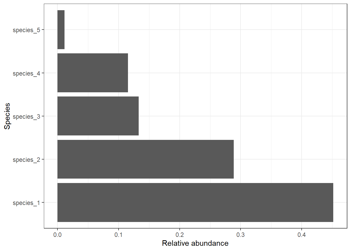
To calculate relative abundance of each species within each site.
# Option 1 - using wide format data
fake_data_clean %>%
  group_by(site) %>%
  summarise(across(starts_with("species_"), sum)) %>%   # total abundance per species per site
  mutate(total = rowSums(across(starts_with("species_")))) %>%  # site-level total abundance
  mutate(across(starts_with("species_"), ~ .x / total)) # divide species abundance by site total
# A tibble: 3 × 7
site species_1 species_2 species_3 species_4 species_5 total
<fct> <dbl> <dbl> <dbl> <dbl> <dbl> <dbl>
1 A 0.571 0.171 0.148 0.109 0 539
2 B 0.418 0.199 0.245 0.113 0.0243 371
3 C 0.350 0.477 0.0352 0.123 0.0137 511# Option 2 - using long format data
relative_site_sum <- fake_data_long %>%
group_by(site, species) %>%
summarise(total_abundance = sum(abundance)) %>%
mutate(site_total = sum(total_abundance),
rel_abundance = total_abundance / site_total)
# Visualise results
relative_site_sum %>%
ggplot() +
geom_bar(aes(x = site, y = rel_abundance, fill = species), stat = "identity", position = position_dodge()) +
labs(x = "Sites", y = "Relative abundance") +
theme_bw()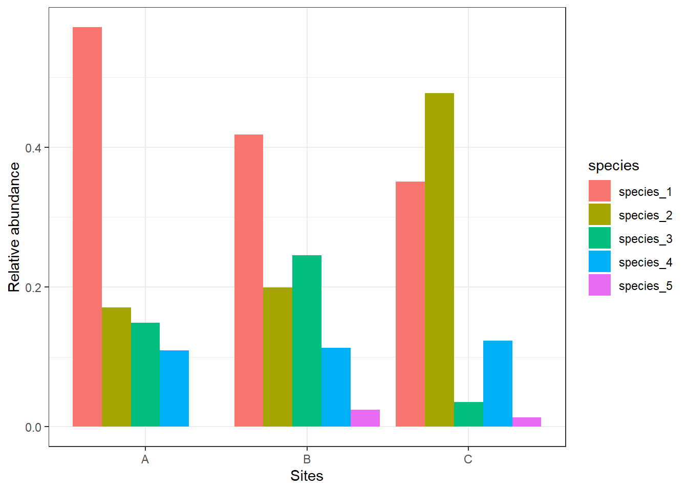
We see that species_1 makes up about 57% of the sample for Site A, and species_4 makes up about 11% of the sample. Once we calculate relative densities for each species at each site, this eliminates differences in total density at each site because all sites then total to 1.
Equation:
\[ d_i = \frac{N_i}{A} \]
where \(d_i\) is the density of species \(i\) (e.g, individuals/ha), \(N_i\) absolute abundance of species \(i\), \(A\) is the area sampled (e.g. m2, ha, km2).
For example, if you counted 42 lizards in a 0.5 ha plot: \(d_i\) = 42/0.5 = 84 individuals/ha.
To calculate density for each site per sampling event (individuals/site/sampling event) in R, here is the following code.
# Option 1 - wide format
fake_data_clean %>%
  group_by(site) %>%
  summarise(round(across(starts_with("species"), mean, na.rm = TRUE))) # calculates the mean count per site across the sampling period.
# A tibble: 3 × 6
site species_1 species_2 species_3 species_4 species_5
<fct> <dbl> <dbl> <dbl> <dbl> <dbl>
1 A 62 18 16 12 0
2 B 31 15 18 8 2
3 C 36 49 4 13 1# Option 2 - long format
density_sum <- fake_data_long %>%
group_by(site, species) %>%
summarise(density = round(mean(abundance))) # calculates the mean count per site across the sampling period.
# Visualise results
density_sum %>%
ggplot() +
geom_bar(aes(x = site, y = density, fill = species), stat = "identity", position = position_dodge()) +
labs(x = "Sites", y = "Density (n/sample effort)") +
theme_bw()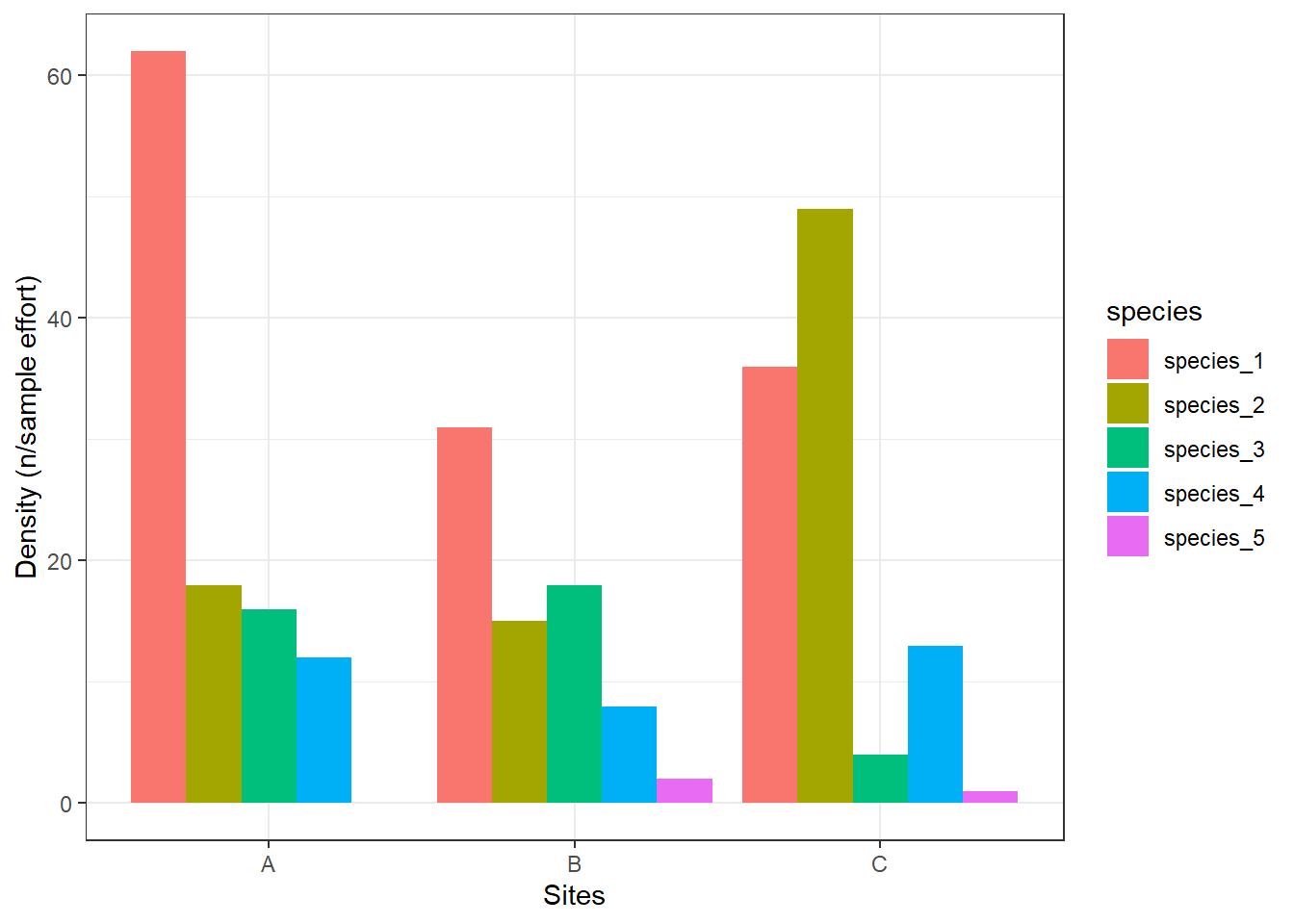
We can see here that site A has 62 individuals per sampling effort for species_1, while site B has 31 indidvuals per sampling effort for species_1.
If you want density of all individuals by site, then use the following code.
fake_data_long %>%
  group_by(site) %>%
  summarise(density = round(mean(abundance))) # calculates the mean count per site across the sampling period.
Site A has an average of 22 individuals per sampling effort, while site B has an average of 20 individuals per sampling effort.
Exercise 1 (10 min)
🧪 Complete the following task for the excerise_survey_data below
- Calculate the absolute abundance, relative abundance, and density of all species by sites
- What is the absolute abundance of species_1 overall?
- What is the relative abundance of species_2 in site B relative to all sampled sites?
- What is the mean density of species_3 overall?
excerise_survey_data <- data.frame(
  site = c("A","A","A","B","B","B","C","C","C"),
  plot = c(1,2,3,1,2,3,1,2,3),
  species_1 = c(12, 7, 15, 4, 9, 6, 20, 18, 25),
  species_2 = c(5, 2, 1, 10, 7, 4, 3, 1, 0),
  species_3 = c(0, 3, 2, 6, 4, 5, 0, 1, 2),
  species_4 = c(8, 6, 3, 1, 4, 2, 10, 7, 5)
)
Show answer
excerise_survey_long <- excerise_survey_data %>%
  tidyr::pivot_longer(!c(site, plot), names_to = "species", values_to = "abundance")# convert wide format to long format (easier to summaries groups)

excerise_survey_sum <- excerise_survey_long %>%
  group_by(site, species) %>% # grouped by site and species
  summarise(species_sum = sum(abundance), # calculates total abundance by site and species (so combination of the plots)
            relative = (species_sum / sum(excerise_survey_long$abundance) * 100), # calculates relative abundance from all species in all sites combined.
            density = round(mean(abundance)) # calculates density (individuals/plot)
            )

# answer 1
excerise_survey_sum %>%
  filter(species == "species_1") %>%
  pull(species_sum) %>%
  sum()

# answer 2
excerise_survey_sum %>%
  filter(species == "species_2", site == "B") %>%
  select(relative)

# answer 3
excerise_survey_sum %>%
  filter(species == "species_3") %>%
  pull(density) %>%
  mean()


# 1. 116
# 2. 10%
# 3. 2.6
Calculations of species richness
Equation:
\[ S = number \, of \, species \, observed \]
To calculate species richness in R, here is the following code. Note, you will need to remove zeros when using length() to count number of species because length will include zero.
# Option 1 - using tidyverse
fake_data_long %>%
  filter(abundance != 0) %>% # remove rows with zeros (e.g. no species 5 in site A)
  group_by(site) %>%
  summarise(total = length(unique(species)))
In our fake dataset, we have four species in site A, and all five species in site B and C. Note, if we includes zeros in this calculation, we would get species_5 in the count which means all sites would have five species, which is incorrect.
Species richness increases with sample size, and differences in richness actually may be caused by differences in sample size. To solve this problem, we may try to rarefy species richness to the same number of individuals.
To calculate absolute abundance of one species in R, here is the following code.
# sum species counts per site
site_counts <- fake_data_clean %>%
  group_by(site) %>%
  summarise(across(where(is.numeric), sum))


# Rarefied richness needs a “sample size” = smallest total abundance across sites.
nmin <- rowSums(site_counts[ , -1]) %>% min()

rarefied_richness_output <- vegan::rarefy(site_counts[ , -1], sample = nmin)

# add rarefied results to sites
rarefied_richness <- bind_cols(site = site_counts$site,
                               rarefied_richness = rarefied_richness_output)
In this fake dataset, the results are the same as your standard species richness count. When you have more complicated and more variable datasets with lots of rare species, this calculation might be useful. Always justify which metric you plan to use in your report.
Exercise 2 (10 min)
🧪 Complete the following task for the excerise_survey_data below
- Calculate the species richness by sites.
- What is the richness of site C?
Show answer
# Species richness
excerise_survey_long %>%
  filter(abundance != 0) %>% # remove rows with zeros (e.g. no species 5 in site A)
  group_by(site) %>%
  summarise(total = length(unique(species)))

# 1. 4
Calculations of diversity
Equation:
\[ H' = - \sum_{i=1}^{S} p_i \,\ln(p_i) \]
where \(H'\) is Shannon diversity index, \(S\) is the total number of species in the community (species richness), \(p_i\) is the relative abundance of species \(i\) (see relative abundance). High \(H'\) = many species, relatively even abundances, while low \(H'\) = few species or dominance by one/few species.
To calculate \(H'\) in R, here is the following code. Note, y
shannon_output <- vegan::diversity(site_counts[, -1], index = "shannon") # remove site column [,-1] for the diversity function to work

# add H results to sites
shannon_sum <- bind_cols(site = site_counts$site,
                               shannon = shannon_output)

# Visualise results
shannon_sum %>%
  ggplot() +
  geom_bar(aes(x = site, y = shannon), stat = "identity") +
  labs(x = "Sites", y = "Shannon diveristy index (H')") +
  theme_bw()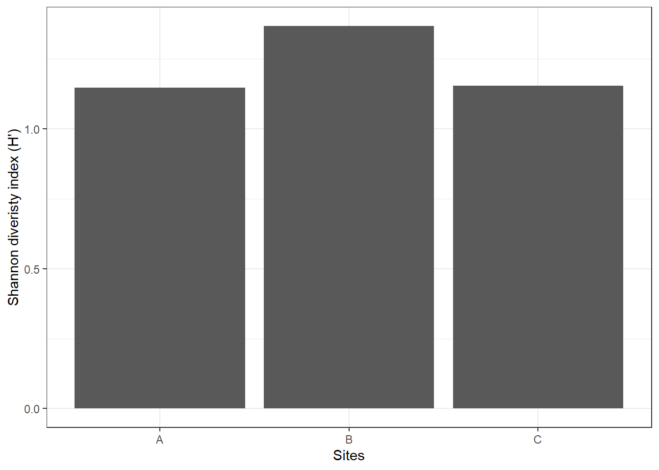
If \(H'\) = 0, only one species is present (no diversity). A value of 1.36 in site B means site B has slighty higher diversity than site A and site C. i.e. more species and/or a more even distribution of individuals among species.
Equation:
\[ D_1 = 1 - \sum_{i=1}^{S} p_i^2 \]
where \(D_1'\) is Simpson’s diversity index, \(S\) is the total number of species in the community (species richness), \(p_i\) is the relative abundance of species \(i\) (see relative abundance). High \(D_1\) = high diversity, while low \(D_1\) = low diversity.
For inverse Simpson’s diversity index, the equation is:
\[ D_2 = \frac{1}{\sum_{i=1}^{S} p_i^2} \] where \(D_2\) is the inverse of Simpson’s diversity index. if \(D_2\) = 1, only one species is present, and if \(D_2\) is higher then more species are present/or more even distribution.
To calculate \(D_1\) in R, here is the following code.
site_counts <- fake_data_clean %>%
  group_by(site) %>%
  summarise(across(where(is.numeric), sum))

# sum species counts per site
simpson_output <- vegan::diversity(site_counts[ , -1], index = "simpson") # remove site column [,-1] for the diversity function to work

# add D1 results to sites
simpson_sum <- bind_cols(site = site_counts$site,
                               simpson = simpson_output)

# Visualise results
simpson_sum %>%
  ggplot() +
  geom_bar(aes(x = site, y = simpson), stat = "identity") +
  labs(x = "Sites", y = "Simpson's diveristy index (D1)") +
  theme_bw()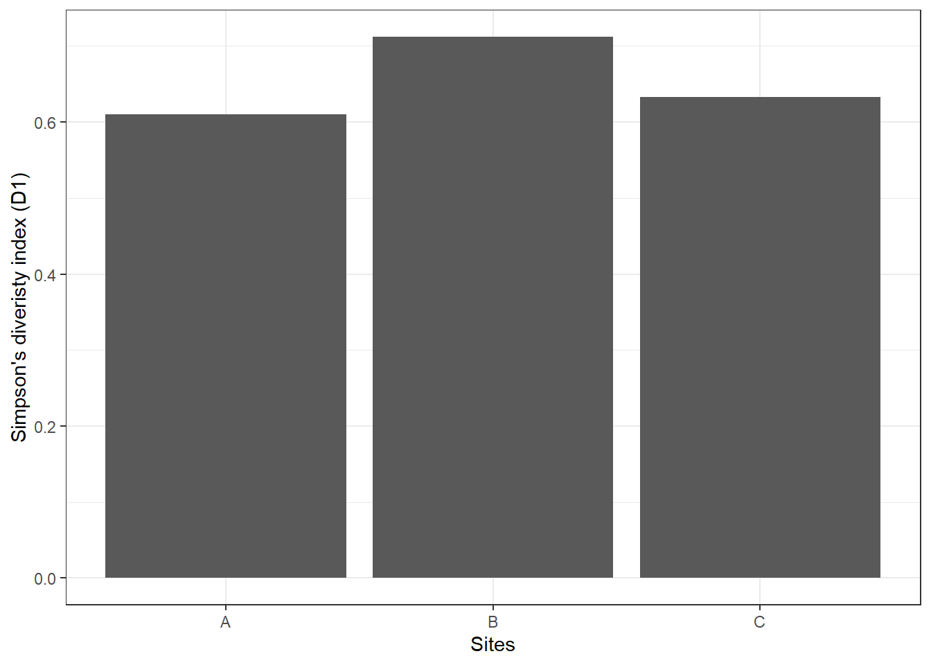
Similar to Shannon diversity index, site B has higher \(D_1\) of 0.71 compared to the other two sites.
Exercise 3 (10 min)
🧪 Complete the following task for the fake_data_clean below
- Calculate the Shannon diversity index, and Simpson’s diversity index by sites (*Note**: Use the original wide format, not long format for this part)
- What is the diversity of site A using the Shannon diversity index (\(H'\)) method?
- What is the diversity of site B using the inverse Simpson’s diversity index (\(D_2\)) method?
Show answer
# sum species counts per site
excerise_survey_sum <- excerise_survey_data %>%
  group_by(site) %>%
  summarise(across(where(is.numeric), sum))

# Shannon diversity
bind_cols(site = excerise_survey_sum$site,
          shannon = vegan::diversity(excerise_survey_sum[, -c(1, 2)], index = "shannon"),
          simpson = vegan::diversity(excerise_survey_sum[, -c(1, 2)], index = "invsimpson"))

# 1. 1.14
# 2. 3.5
Assessment
Task to complete before the end of the workshop.
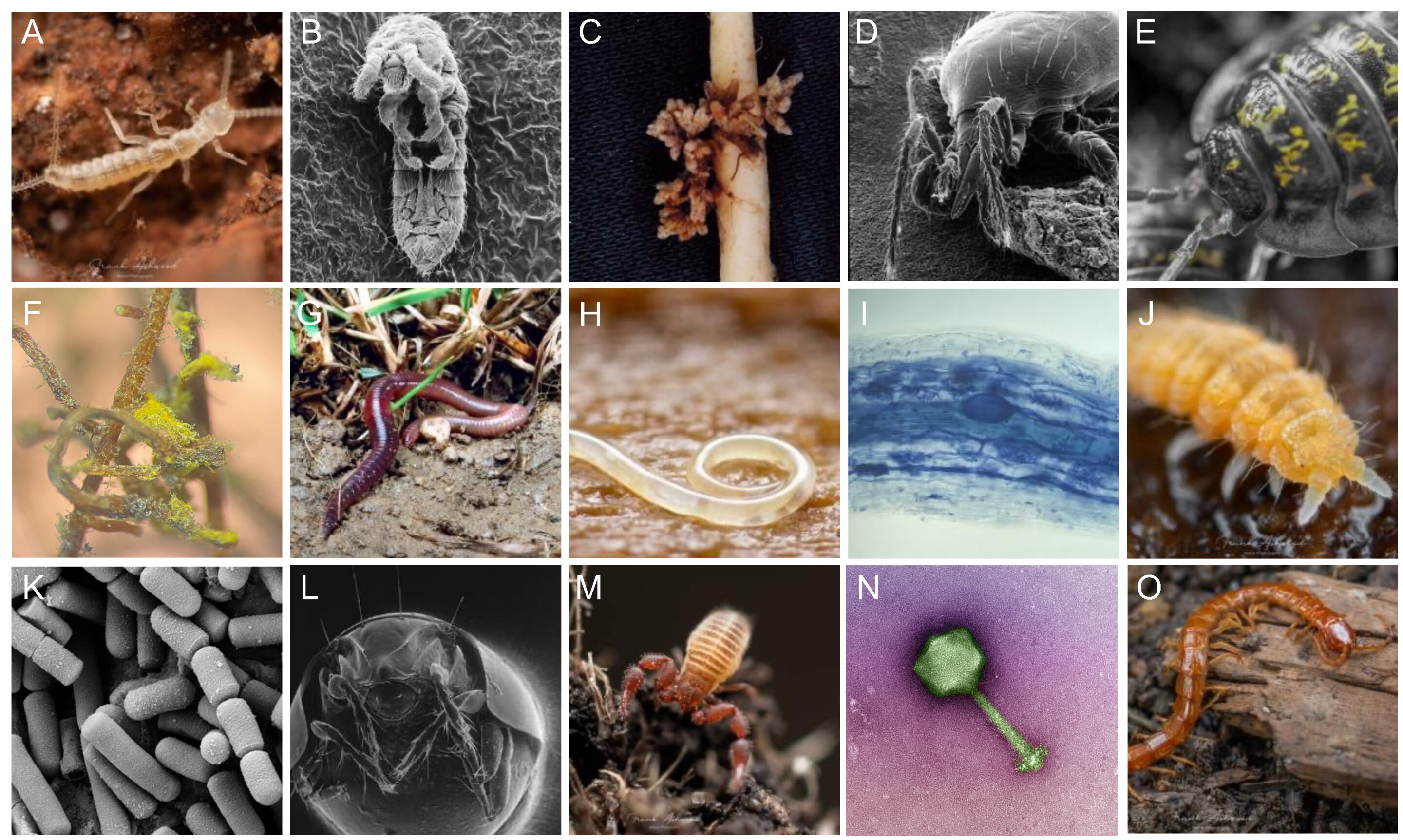
Here is an example from a real dataset looking at the effects of experimental drought on soil invertebrate communities, called invert_exp_survey.csv (Farkas et al., 2025). The invert_exp_survey.csv file can be found on GitHub in the ‘data’ folder.
The invertebrate diversity is grouped at order level, with the exception of Crustacea (subphylum), Diplopoda (class), Chilopoda (class), and Annelida (phylum).
Use the skills that you learnt in the previous practical and this weeks practical to complete the following assessment with the example dataset invert_exp_survey.csv:
1. Load data and inspect structure
- Create a working for your
invert_exp_survey.csvdata - Import
invert_exp_survey.csvinto R - Inspect the structure and column names
- Check for missing values
- Check for duplicate rows
# Week 3 workshop - Diversity
# Written by Nicholas Wu, 06/11/2024, Murdoch University

# Load packages
library(tidyverse)
library(visdat)

# Set your working directory
setwd("YOUR-DIRECTORY")

# Load your data
invert_raw <- read_csv("invert_exp_survey.csv")

# Convert to long format
2. Calculate and visualise relative abundance by treatment (i.e, Within each treatment, what proportion of the total community does each invertebrate order make up?)
- Sum the total abundance of each order by treatment. Hint: use Option 2 - using long format data (one row per sample × order)
- The figure should look close to this.
# QUESTION 2: What proportion of the total community does each invertebrate order make up?


# Plot the summarised outcome
rel_abund %>%
  ggplot() +
  geom_bar(
    aes(x = order, y = rel_abundance, fill = treatment),
    stat = "identity",
    position = position_dodge()
  ) +
  labs(x = NULL, y = "Relative abundance") +
  theme_bw() +
  coord_flip()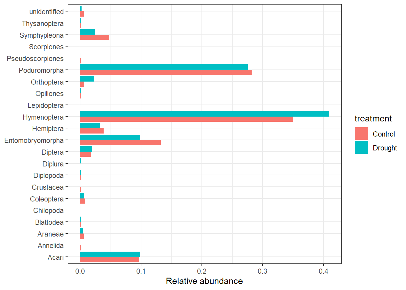
3. Calculate species richness per treatment
- Count the number of unique invertebrate orders with abundance > 0
4. Calculate Shannon diversity index by treatment
- You can find the code to summarise species counts per site under the ‘rarified species’ section (
site_counts). - Apply
vegan::diversity() - Apply
bind_cols()to match the shannon numbers with your treatment names. - Plot it, the figure should look close to this.
shannon_inv %>%
  ggplot() +
  geom_bar(
    aes(x = treatment, y = shannon),
    stat = "identity"
  ) +
  labs(x = "Treatment", y = "Shannon diveristy index (H')") +
  theme_bw()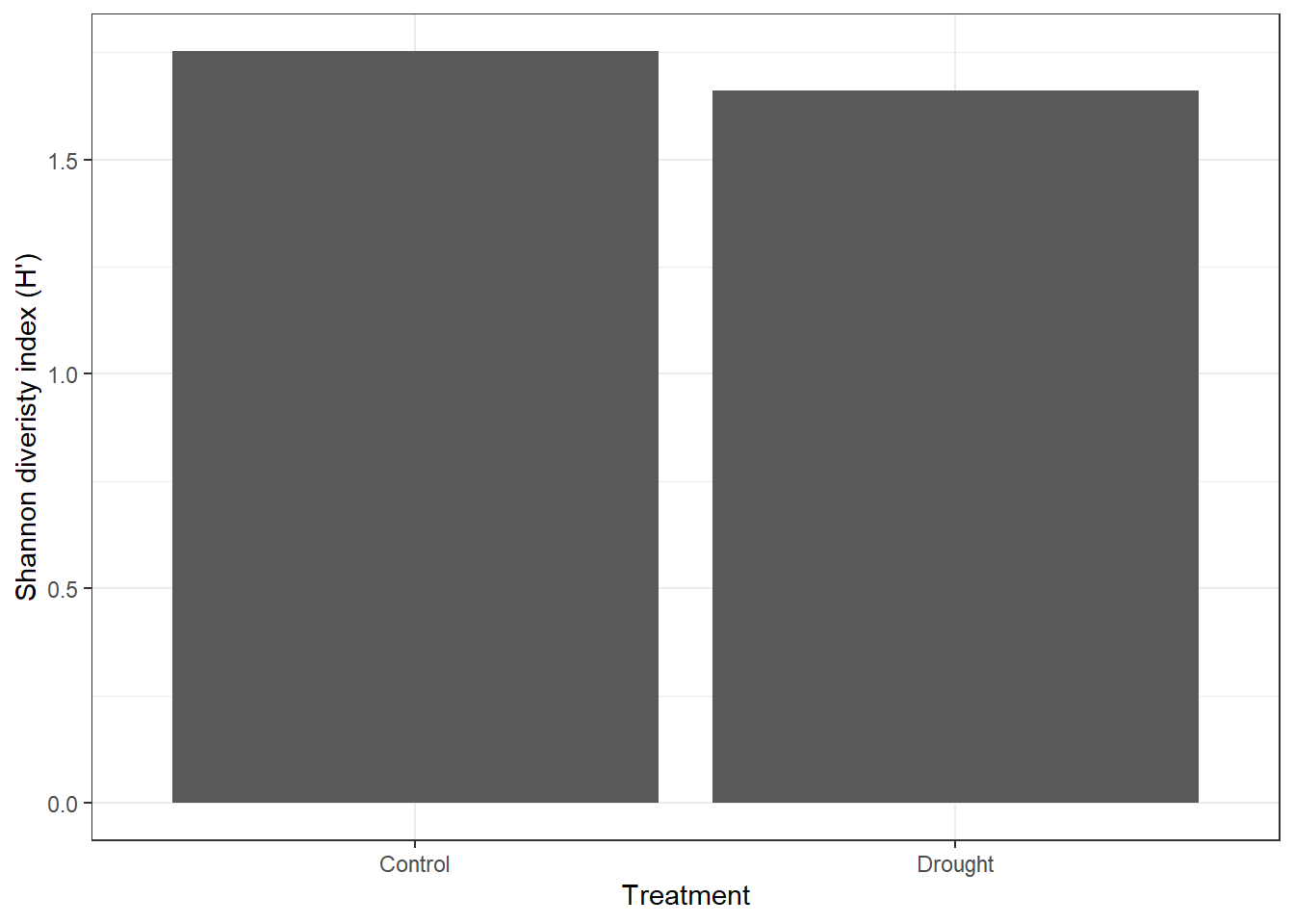
For the adventurous folks
Try to get Shannon diversity index by treatment and block. Convert wide data to sums per treatment x block.
See if you can replicate this figure.
shannon_inv %>%
  ggplot() +
  geom_point(aes(x = treatment, y = shannon), size = 2) +
  labs(x = "Treatment", y = "Shannon diveristy index (H')") +
  theme_bw()
This is more reflective of the normal variation across experimental blocks and where your report should be going towards instead ot the mean only.
Extra Stuff
- More detailed background and theory on indices of diversity and evenness with example R code and dataset to play with.